The NLP Procedure

Example 7.9 Minimize Total Delay in a Network

The following example is taken from the user’s guide of GINO (Liebman et al. 1986). A simple network of five roads (arcs) can be illustrated by the path diagram:

Output 7.9.1: Simple Road Network

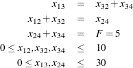
The five roads connect four intersections illustrated by numbered nodes. Each minute F vehicles enter and leave the network. Arc $(i,j)$ refers to the road from intersection i to intersection j, and the parameter $x_{ij}$ refers to the flow from i to j. The law that traffic flowing into each intersection j must also flow out is described by the linear equality constraint

$\sum _ i x_{ij} = \sum _ i x_{ji} \: , \quad j=1,\ldots ,n$

In general, roads also have an upper capacity, which is the number of vehicles which can be handled per minute. The upper limits $c_{ij}$ can be enforced by boundary constraints

$0 \le x_{ij} \le c_{ij} \: , \quad i,j=1,\ldots ,n$

Finding the maximum flow through a network is equivalent to solving a simple linear optimization problem, and for large problems, PROC LP or PROC NETFLOW can be used. The objective function is

$\max \quad f = x_{24} + x_{34}$

and the constraints are

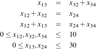
$\begin{eqnarray*} x_{13} & = & x_{32} + x_{34} \\ x_{12} + x_{32} & = & x_{24} \\ x_{12} + x_{13} & = & x_{24} + x_{34} \\ 0 \le x_{12}, x_{32}, x_{34} & \le & 10 \\ 0 \le x_{13}, x_{24} & \le & 30 \end{eqnarray*}$

The three linear equality constraints are linearly dependent. One of them is deleted automatically by the PROC NLP subroutines. Even though the default technique is used for this small example, any optimization subroutine can be used.

proc nlp all initial=.5;
   max y;
   parms x12 x13 x32 x24 x34;
   bounds x12 <= 10,
          x13 <= 30,
          x32 <= 10,
          x24 <= 30,
          x34 <= 10;
   /* what flows into an intersection must flow out */
   lincon x13 = x32 + x34,
          x12 + x32 = x24,
          x24 + x34 = x12 + x13;
   y = x24 + x34 + 0*x12 + 0*x13 + 0*x32;
run;

The iteration history is given in Output 7.9.2, and the optimal solution is given in Output 7.9.3.

Output 7.9.2: Iteration History

PROC NLP: Nonlinear Maximization

Newton-Raphson Ridge Optimization

Without Parameter Scaling

Iteration		Restarts	Function Calls	Active Constraints		Objective Function	Objective Function Change	Max Abs Gradient Element	Ridge	Ratio Between Actual and Predicted Change
1	*	0	2	4		20.25000	19.2500	0.5774	0.0313	0.860
2	*	0	3	5		30.00000	9.7500	0	0.0313	1.683

Optimization Results
Iterations	2	Function Calls	4
Hessian Calls	3	Active Constraints	5
Objective Function	30	Max Abs Gradient Element	0
Ridge	0	Actual Over Pred Change	1.6834532374

All parameters are actively constrained. Optimization cannot proceed.

Output 7.9.3: Optimization Results

PROC NLP: Nonlinear Maximization

Optimization Results
Parameter Estimates
N	Parameter	Estimate	Gradient Objective Function	Active Bound Constraint
1	x12	10.000000	0	Upper BC
2	x13	20.000000	0
3	x32	10.000000	0	Upper BC
4	x24	20.000000	1.000000
5	x34	10.000000	1.000000	Upper BC

Value of Objective Function = 30

Finding a traffic pattern that minimizes the total delay to move F vehicles per minute from node 1 to node 4 introduces nonlinearities that, in turn, demand nonlinear optimization techniques. As traffic volume increases, speed decreases. Let $t_{ij}$ be the travel time on arc $(i,j)$ and assume that the following formulas describe the travel time as decreasing functions of the amount of traffic:

$\begin{eqnarray*} t_{12} & = & 5 + 0.1 x_{12} / (1 - x_{12}/10) \\ t_{13} & = & x_{13} / (1 - x_{13}/30) \\ t_{32} & = & 1 + x_{32} / (1 - x_{32}/10) \\ t_{24} & = & x_{24} / (1 - x_{24}/30) \\ t_{34} & = & 5 + 0.1 x_{34} / (1 - x_{34}/10) \end{eqnarray*}$

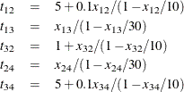
These formulas use the road capacities (upper bounds), assuming $F=5$ vehicles per minute have to be moved through the network. The objective function is now

$\min \quad f = t_{12} x_{12} + t_{13} x_{13} + t_{32} x_{32} + t_{24} x_{24} + t_{34} x_{34}$

and the constraints are

$\begin{eqnarray*} x_{13} & = & x_{32} + x_{34} \\ x_{12} + x_{32} & = & x_{24} \\ x_{24} + x_{34} & = & F = 5 \\ 0 \le x_{12}, x_{32}, x_{34} & \le & 10 \\ 0 \le x_{13}, x_{24} & \le & 30 \end{eqnarray*}$

Again, the default algorithm is used:

proc nlp all initial=.5;
   min y;
   parms x12 x13 x32 x24 x34;
   bounds x12 x13 x32 x24 x34 >= 0;
   lincon x13 = x32 + x34,  /* flow in = flow out */
          x12 + x32 = x24,
          x24 + x34 = 5;    /* = f = desired flow */
   t12 = 5 + .1 * x12 / (1 - x12 / 10);
   t13 = x13 / (1 - x13 / 30);
   t32 = 1 + x32 / (1 - x32 / 10);
   t24 = x24 / (1 - x24 / 30);
   t34 = 5 + .1 * x34 / (1 - x34 / 10);
   y = t12*x12 + t13*x13 + t32*x32 + t24*x24 + t34*x34;
run;

The iteration history is given in Output 7.9.4, and the optimal solution is given in Output 7.9.5.

Output 7.9.4: Iteration History

PROC NLP: Nonlinear Minimization

Newton-Raphson Ridge Optimization

Without Parameter Scaling

Iteration		Restarts	Function Calls	Active Constraints		Objective Function	Objective Function Change	Max Abs Gradient Element	Ridge	Ratio Between Actual and Predicted Change
1		0	2	4		40.30303	0.3433	4.44E-16	0	0.508

Optimization Results
Iterations	1	Function Calls	3
Hessian Calls	2	Active Constraints	4
Objective Function	40.303030303	Max Abs Gradient Element	4.440892E-16
Ridge	0	Actual Over Pred Change	0.5083585587

ABSGCONV convergence criterion satisfied.

Output 7.9.5: Optimization Results

PROC NLP: Nonlinear Minimization

Optimization Results
Parameter Estimates
N	Parameter	Estimate	Gradient Objective Function	Active Bound Constraint
1	x12	2.500000	5.777778
2	x13	2.500000	5.702479
3	x32	1.114018E-17	1.000000	Lower BC
4	x24	2.500000	5.702479
5	x34	2.500000	5.777778

Value of Objective Function = 40.303030303

The active constraints and corresponding Lagrange multiplier estimates (costs) are given in Output 7.9.6 and Output 7.9.7, respectively.

Output 7.9.6: Linear Constraints at Solution

PROC NLP: Nonlinear Minimization

Linear Constraints Evaluated at Solution
1	ACT	4.4409E-16	=	0	+	1.0000	*	x13	-	1.0000	*	x32	-	1.0000	*	x34
2	ACT	4.4409E-16	=	0	+	1.0000	*	x12	+	1.0000	*	x32	-	1.0000	*	x24
3	ACT	0	=	-5.0000	+	1.0000	*	x24	+	1.0000	*	x34

Output 7.9.7: Lagrange Multipliers at Solution

PROC NLP: Nonlinear Minimization

First Order Lagrange Multipliers
Active Constraint		Lagrange Multiplier
Lower BC	x32	0.924702
Linear EC	[1]	5.702479
Linear EC	[2]	5.777778
Linear EC	[3]	11.480257

Output 7.9.8 shows that the projected gradient is very small, satisfying the first-order optimality criterion.

Output 7.9.8: Projected Gradient at Solution

PROC NLP: Nonlinear Minimization

Projected Gradient
Free Dimension	Projected Gradient
1	4.440892E-16

The projected Hessian matrix (shown in Output 7.9.9) is positive definite, satisfying the second-order optimality criterion.

Output 7.9.9: Projected Hessian at Solution

PROC NLP: Nonlinear Minimization

Projected Hessian Matrix
	X1
X1	1.535309013