For generalized networks you can specify either EXCESS=SUPPLY or EXCESS=DEMAND to indicate which nodal flow conservation constraints have slack variables associated with them. The default option is EXCESS=NONE.
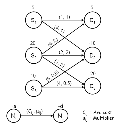
Consider the simple network shown in Output 6.11.1. As you can see, the sum of positive supdem values (35) is equal to the absolute sum of the negative ones. However, the arcs connecting the supply and demand nodes have
varying arc multipliers. Let us now solve the problem using the EXCESS=SUPPLY option.
You can use the following SAS code to create the input data sets:
data garcs;
   input _from_ $ _to_ $ _cost_ _mult_;
datalines;
s1 d1 1 .
s1 d2 8 .
s2 d1 4 2
s2 d2 2 2
s2 d3 1 2
s3 d2 5 0.5
s3 d3 4 0.5
;

data gnodes;
   input _node_ $ _sd_ ;
datalines;
s1  5
s2  20
s3  10
d1  -5
d2  -10
d3  -20
;
To solve the problem, use the following call to PROC NETFLOW:
title1 'The NETFLOW Procedure';
proc netflow
   arcdata  = garcs
   nodedata = gnodes
   excess   = supply
   conout   = gnetout;
run;
The optimal solution is displayed in Output 6.11.2.
Output 6.11.2: Optimal Solution Obtained Using the EXCESS=SUPPLY Option
| The NETFLOW Procedure |
| Obs | _from_ | _to_ | _cost_ | _CAPAC_ | _LO_ | _mult_ | _SUPPLY_ | _DEMAND_ | _FLOW_ | _FCOST_ |
|---|---|---|---|---|---|---|---|---|---|---|
| 1 | s1 | d1 | 1 | 99999999 | 0 | 1.0 | 5 | 5 | 5 | 5 |
| 2 | s2 | d1 | 4 | 99999999 | 0 | 2.0 | 20 | 5 | 0 | 0 |
| 3 | s1 | d2 | 8 | 99999999 | 0 | 1.0 | 5 | 10 | 0 | 0 |
| 4 | s2 | d2 | 2 | 99999999 | 0 | 2.0 | 20 | 10 | 5 | 10 |
| 5 | s3 | d2 | 5 | 99999999 | 0 | 0.5 | 10 | 10 | 0 | 0 |
| 6 | s2 | d3 | 1 | 99999999 | 0 | 2.0 | 20 | 20 | 10 | 10 |
| 7 | s3 | d3 | 4 | 99999999 | 0 | 0.5 | 10 | 20 | 0 | 0 |
Note: If you do not specify the EXCESS= option, or if you specify the EXCESS=DEMAND option, the procedure will declare the problem infeasible. Therefore, in case of real-life problems, you would need to have a little more detail about how the arc multipliers end up affecting the network — whether they tend to create excess demand or excess supply.
Consider the previous example but with a slight modification: the arcs out of node ![]() have multipliers of 0.5, and the arcs out of node
have multipliers of 0.5, and the arcs out of node ![]() have multipliers of 1. You can use the following SAS code to create the input arc data set:
have multipliers of 1. You can use the following SAS code to create the input arc data set:
data garcs1;
   input _from_ $ _to_ $ _cost_ _mult_;
datalines;
s1 d1 1 0.5
s1 d2 8 0.5
s2 d1 4 .
s2 d2 2 .
s2 d3 1 .
s3 d2 5 0.5
s3 d3 4 0.5
;
Note that the node data set remains unchanged. You can use the following call to PROC NETFLOW to solve the problem:
title1 'The NETFLOW Procedure';
proc netflow
   arcdata  = garcs1
   nodedata = gnodes
   excess = demand
   conout   = gnetout1;
run;
The optimal solution is displayed in Output 6.11.3.
Output 6.11.3: Optimal Solution Obtained Using the EXCESS=DEMAND Option
| The NETFLOW Procedure |
| Obs | _from_ | _to_ | _cost_ | _CAPAC_ | _LO_ | _mult_ | _SUPPLY_ | _DEMAND_ | _FLOW_ | _FCOST_ |
|---|---|---|---|---|---|---|---|---|---|---|
| 1 | s1 | d1 | 1 | 99999999 | 0 | 0.5 | 5 | 5 | 5.0000 | 5.0000 |
| 2 | s2 | d1 | 4 | 99999999 | 0 | 1.0 | 20 | 5 | 0.0000 | 0.0000 |
| 3 | s1 | d2 | 8 | 99999999 | 0 | 0.5 | 5 | 10 | 0.0000 | 0.0000 |
| 4 | s2 | d2 | 2 | 99999999 | 0 | 1.0 | 20 | 10 | 5.0000 | 10.0000 |
| 5 | s3 | d2 | 5 | 99999999 | 0 | 0.5 | 10 | 10 | 0.0000 | 0.0000 |
| 6 | s2 | d3 | 1 | 99999999 | 0 | 1.0 | 20 | 20 | 15.0000 | 15.0000 |
| 7 | s3 | d3 | 4 | 99999999 | 0 | 0.5 | 10 | 20 | 10.0000 | 40.0000 |