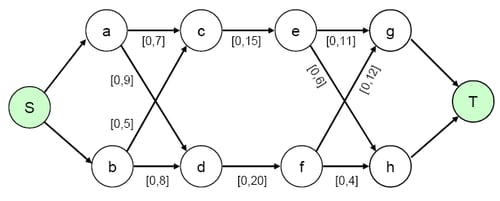
Consider the maximum flow problem depicted in Output 6.10.1. The maximum flow between nodes S and T is to be determined. The minimum arc flow and arc capacities are specified as lower and upper bounds in square brackets, respectively.
You can solve the problem using either EXCESS=ARCS or EXCESS=SLACKS. Consider using the EXCESS=ARCS option first. You can use the following SAS code to create the input data set:
data arcs;
   input _from_ $ _to_ $ _cost_ _capac_;
datalines;
S a  .  .
S b  .  .
a c  1  7
b c  2  9
a d  3  5
b d  4  8
c e  5 15
d f  6 20
e g  7 11
f g  8  6
e h  9 12
f h 10  4
g T  .  .
h T  .  .
;
You can use the following call to PROC NETFLOW to solve the problem:
title1 'The NETFLOW Procedure';
proc netflow
   intpoint
   maxflow
   excess = arcs
   arcdata = arcs
   source  = S    sink = T
   conout  = gout3;
run;
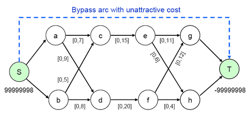
With the EXCESS=ARCS option specified, the problem gets transformed internally to the one depicted in Output 6.10.2. Note that there is an additional arc from the source node to the sink node.
The output SAS data set is displayed in Output 6.10.3.
Output 6.10.3: Maximum Flow Problem, EXCESS=ARCS Option Specified
| The NETFLOW Procedure |
| Obs | _from_ | _to_ | _cost_ | _capac_ | _LO_ | _SUPPLY_ | _DEMAND_ | _FLOW_ | _FCOST_ |
|---|---|---|---|---|---|---|---|---|---|
| 1 | g | T | 0 | 99999999 | 0 | . | 99999998 | 16.9996 | 0.0000 |
| 2 | h | T | 0 | 99999999 | 0 | . | 99999998 | 8.0004 | 0.0000 |
| 3 | S | a | 0 | 99999999 | 0 | 99999998 | . | 11.9951 | 0.0000 |
| 4 | S | b | 0 | 99999999 | 0 | 99999998 | . | 13.0049 | 0.0000 |
| 5 | a | c | 1 | 7 | 0 | . | . | 6.9952 | 6.9952 |
| 6 | b | c | 2 | 9 | 0 | . | . | 8.0048 | 16.0097 |
| 7 | a | d | 3 | 5 | 0 | . | . | 4.9999 | 14.9998 |
| 8 | b | d | 4 | 8 | 0 | . | . | 5.0001 | 20.0002 |
| 9 | c | e | 5 | 15 | 0 | . | . | 15.0000 | 75.0000 |
| 10 | d | f | 6 | 20 | 0 | . | . | 10.0000 | 60.0000 |
| 11 | e | g | 7 | 11 | 0 | . | . | 10.9996 | 76.9975 |
| 12 | f | g | 8 | 6 | 0 | . | . | 6.0000 | 48.0000 |
| 13 | e | h | 9 | 12 | 0 | . | . | 4.0004 | 36.0032 |
| 14 | f | h | 10 | 4 | 0 | . | . | 4.0000 | 40.0000 |
You can solve the same maximum flow problem, but this time with EXCESS=SLACKS specified. The SAS code is as follows:
title1 'The NETFLOW Procedure';
proc netflow
   intpoint
   excess  = slacks
   arcdata = arcs
   source  = S    sink = T
   maxflow
   conout  = gout3b;
run;
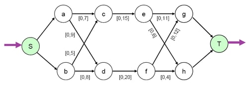
With the EXCESS=SLACKS option specified, the problem gets transformed internally to the one depicted in Output 6.10.4. Note that the source node and sink node each have a single-ended “excess” arc attached to them.
The solution, as displayed in Output 6.10.5, is the same as before. Note that the _SUPPLY_ value of the source node Y has changed from 99999998 to missing S, and the _DEMAND_value of the sink node Z has changed from ![]() 99999998 to missing D.
99999998 to missing D.
Output 6.10.5: Maximal Flow Problem
| The NETFLOW Procedure |
| Obs | _from_ | _to_ | _cost_ | _capac_ | _LO_ | _SUPPLY_ | _DEMAND_ | _FLOW_ | _FCOST_ |
|---|---|---|---|---|---|---|---|---|---|
| 1 | g | T | 0 | 99999999 | 0 | . | D | 16.9993 | 0.0000 |
| 2 | h | T | 0 | 99999999 | 0 | . | D | 8.0007 | 0.0000 |
| 3 | S | a | 0 | 99999999 | 0 | S | . | 11.9867 | 0.0000 |
| 4 | S | b | 0 | 99999999 | 0 | S | . | 13.0133 | 0.0000 |
| 5 | a | c | 1 | 7 | 0 | . | . | 6.9868 | 6.9868 |
| 6 | b | c | 2 | 9 | 0 | . | . | 8.0132 | 16.0264 |
| 7 | a | d | 3 | 5 | 0 | . | . | 4.9999 | 14.9998 |
| 8 | b | d | 4 | 8 | 0 | . | . | 5.0001 | 20.0002 |
| 9 | c | e | 5 | 15 | 0 | . | . | 15.0000 | 75.0000 |
| 10 | d | f | 6 | 20 | 0 | . | . | 10.0000 | 60.0000 |
| 11 | e | g | 7 | 11 | 0 | . | . | 10.9993 | 76.9953 |
| 12 | f | g | 8 | 6 | 0 | . | . | 6.0000 | 48.0000 |
| 13 | e | h | 9 | 12 | 0 | . | . | 4.0007 | 36.0061 |
| 14 | f | h | 10 | 4 | 0 | . | . | 4.0000 | 40.0000 |