Building a Cube from a Summary Table

Overview

In this example, you build a cube with fully summarized data. A summary table is a data source that contains a crossing of all dimensions for a cube. In this example, the summary table PRDNWYPR contains sales data from a furniture company. The table contains columns for location, sales, date, and product values. It also contains stored measures for actual and predicted sales figures.

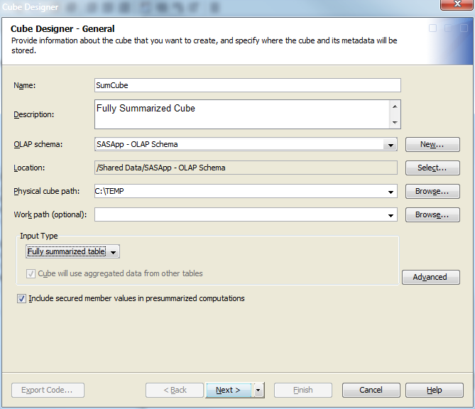
Enter General Cube Information

After you have established a connection profile, you can begin to create a cube. Select File

New

Cube. On the Cube Designer – General page, enter the basic cube information. For this example input type, you click Fully Summarized Table. The following display shows fields that you enter information for.

Enter information in the following fields:
- Name
- Description
- OLAP schema
- Location (SAS folder)
- Physical cube path (path in the file system to store the cube)
- Work path (path for temporary work files)
- Input Type (fully summarized table)

Note: When the Fully summarized table input type is selected, the option Cube will use aggregated data from other tables is automatically selected.

Select an Input Table

Overview

On the Cube Designer – Input page, select an input table for your cube. If one does not exist for your data, click Register Table, and then define the source that you will import your metadata from.

Drill-Through Table

In the Cube Designer – Input page, you can also select or define an optional drill-through table. Drill-through tables can be used by client applications to provide a view from processed data into the underlying source data.

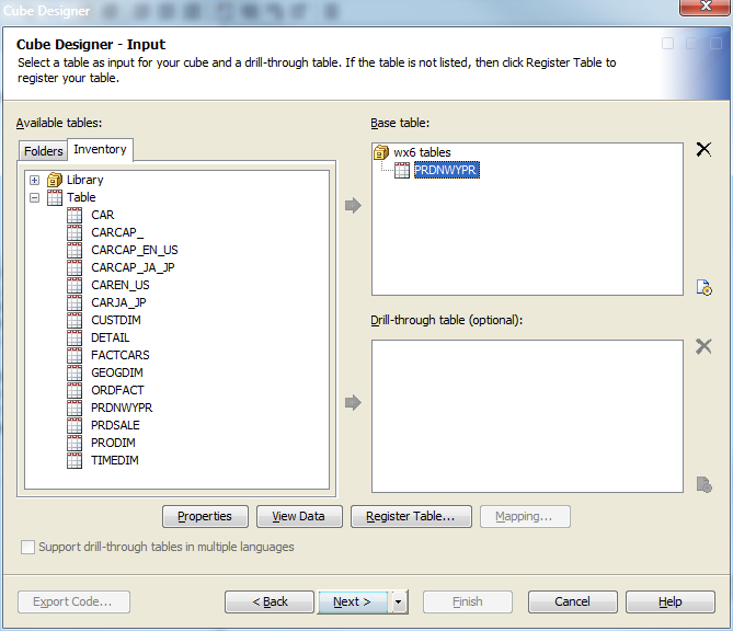
If a drill-through table does not exist for your data, click Register Table.

The following display shows how the summarized table PRDNWYPR is selected for the example cube. No drill-through table has been selected.

Table Options

On the Cube Designer – Input page, you can specify data set options that are used to open either the detail table or drill-through table for your cube. The Table Options button

button near the Base table tree or the Drill-thru table tree is available in both the Cube Designer – Input and the Cube Designer – Drill-Through dialog boxes. The button opens the Table Options dialog box. It enables you to specify data set options that are used to open the data set. For example, you could enter a WHERE clause or subsetting information that is then applied to the selected table when it is opened. The options are stored as part of the cube and then reapplied when the data is accessed at run time. You can also specify data set options in the Dimension Designer – General dialog box (for use with star schemas) and the Stored Aggregates dialog box (for use with summarized tables). For more information, see “Data Set Options” in the SAS Language Reference: Concepts.

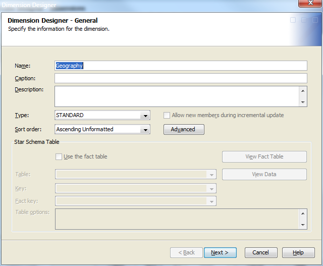
Define Dimensions, Levels, and Hierarchies

Now that your basic metadata server and cube information has been entered, you can define the different dimensions and their respective levels and hierarchies. For this example, the following dimensions are created:

Products
Dates
Geography

On the Cube Designer – Dimensions page, click Add New Dimension. This displays the Dimension Designer – General page, as shown in the following display.

Enter information in the following fields:

Name
Caption
Description
Type (Standard, GEO, or TIME)
Sort order

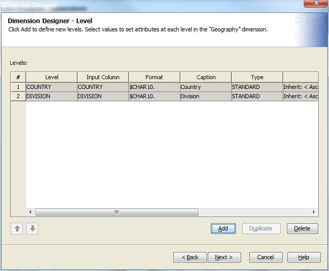
Select Next. This opens the Dimension Designer – Level page. Next, click Add to open the Add Levels dialog box, as shown in the following display.

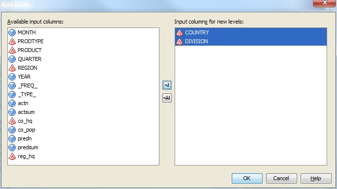
Select the levels that you want to add to the dimension. Select OK to return to the Level page, where the selected levels are listed. You can now define properties such as format, time type, and sort order for the levels that you have selected. See the following display.

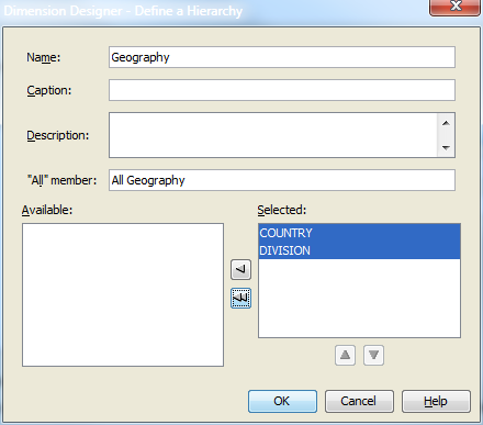
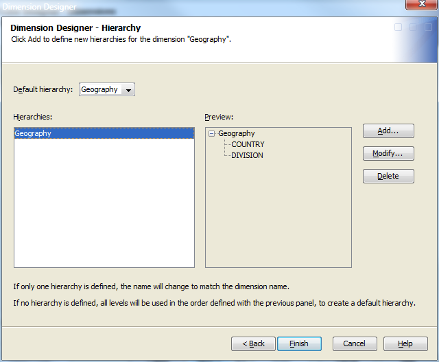
Next, define hierarchies for the levels on the Dimension Designer – Hierarchy page. You can click Add to open the Define a Hierarchy page and individually select the levels for the hierarchy.

Or you can click Finish to accept the order of the levels that are defined on the previous Dimension Designer – Level page. If you select this option, the hierarchy is assigned the same name as the dimension. See the following display.

Repeat this process for each dimension. For this example, the following dimensions are created:

Geography: (levels: Country, Division)
Products: (levels: Product, Product Type)
Dates: (Year, Quarter, Month)

After you create each dimension it is listed in the Dimensions panel of the Cube Designer – Dimensions page. See the following display:

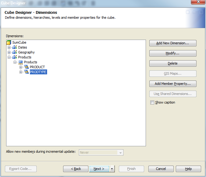
Define Member Properties

You can now define the member properties for any needed cube members. A member property is an attribute of a dimension member. A member property is also an optional cube feature that is created in a dimension to provide users with additional information about members. Define member properties in the Cube Designer – Dimensions page by selecting a level, and then selecting Add Member Property.

Define Measures

Overview

For this example, stored measures and derived measures are created. Stored measures are base measures that are loaded from the fully summarized table. When you are creating a cube from a fully summarized table, the table must have one column for each stored measure in your cube. The base statistics are SUM, N, MIN, MAX, NMISS, and USS.

Derived measures are measures that are built from the stored measures that you have selected for the cube. Derived measures are assigned to an analysis group when they are created. An analysis group is used to identify the numeric column in the original unsummarized data source that was used as the analysis variable for the stored measure. It can also be a name that identifies a logical association between several stored measures.

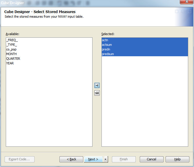
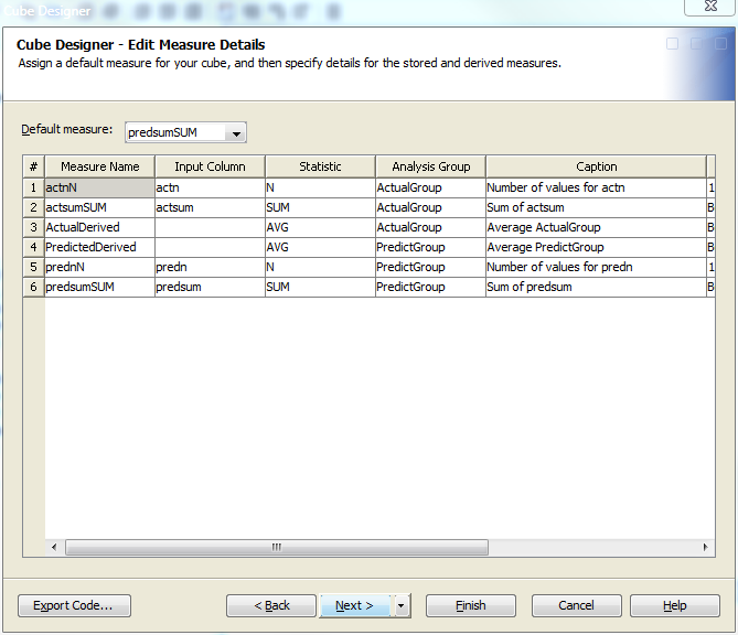
Note: For further information about measure statistics, see Statistics Available for Measures .

Stored Measures

You can now select the stored (base) measures for the cube in the Cube Designer – Select Stored Measures page. From the list of available measures, select the stored measures that you want to include in the cube. For this example actn, actsum, predn, and predsum are included.

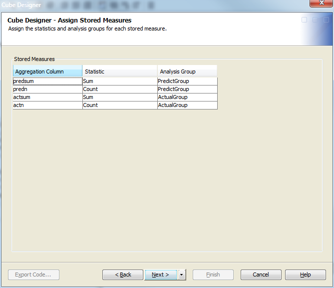
On the Cube Designer – Assign Stored Measures page, you can specify the Statistic and Analysis Group options for the stored measures. For the Statistic, select the appropriate statistic from the drop-down menu. For the Analysis Group, enter a name that identifies a logical association between the stored measures. The Analysis Group name can identify the numeric column in the original unsummarized data source that was used as the analysis variable for the stored measure. If the table contained two measures from the same analysis column, both of the base measures should have the same analysis group specified.

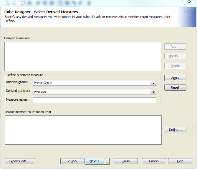
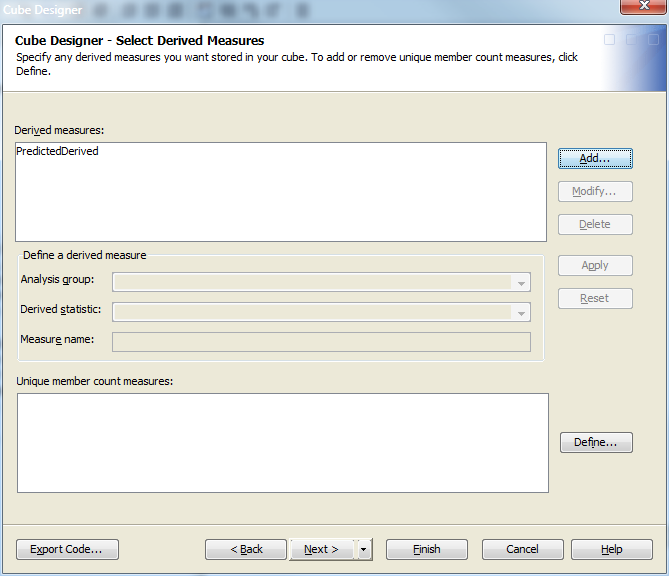
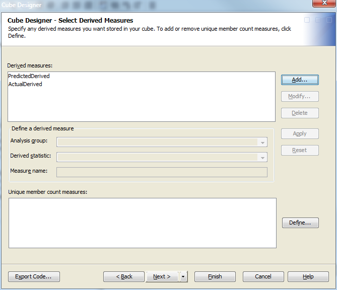
Derived Measures

On the Cube Designer – Select Derived Measures page, specify the measures that are derived from the stored measures. Each derived measure is based on a set of required stored measures. If the stored measures for an analysis group do not include all those required for a specific derived measure, then that measure cannot be included in the cube. On the Define a derived measure panel, select the Analysis group, Derived statistic, and Measure name for the derived measure that you are creating.

When you are finished, click Apply. The derived measure is listed in the Derived Measures list.

For this example, two derived measures are created: ActualDerived and Predicted Derived.

Edit Measure Details

On the Cube Designer – Edit Measure Details page, you can select a default measure and modify measure details for the stored and derived measures.

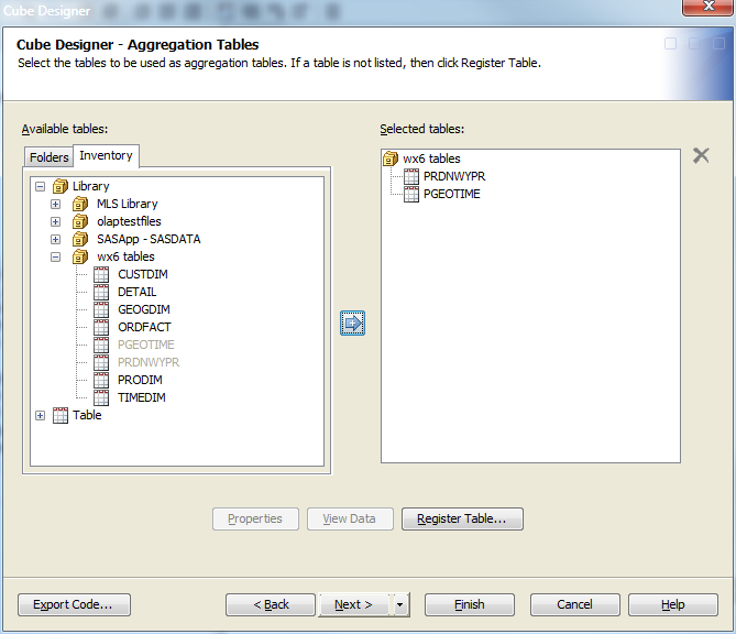
Define Aggregation Tables

On the Cube Designer – Aggregation Tables page, you associate aggregation tables with the summarized data source that you specified as the input data source for the cube. When you open the Cube Designer – Aggregation Tables page, the input data table that you selected to build your cube with is listed in the Selected tables list. You can then select a table to use as the aggregation table from the Available tables list and move it to the Selected tables list. For this example, the table PGEOTIME is used as the aggregation table.

Note: If the cube is loaded from a fully summarized data source, then the measure names within the selected aggregation tables must match the measure names in the input data source. If the cube is loaded from a detail table or a star schema, then all of the selected aggregation tables must use the same measure names. For all cubes, the levels must be the same as those in the input data source.

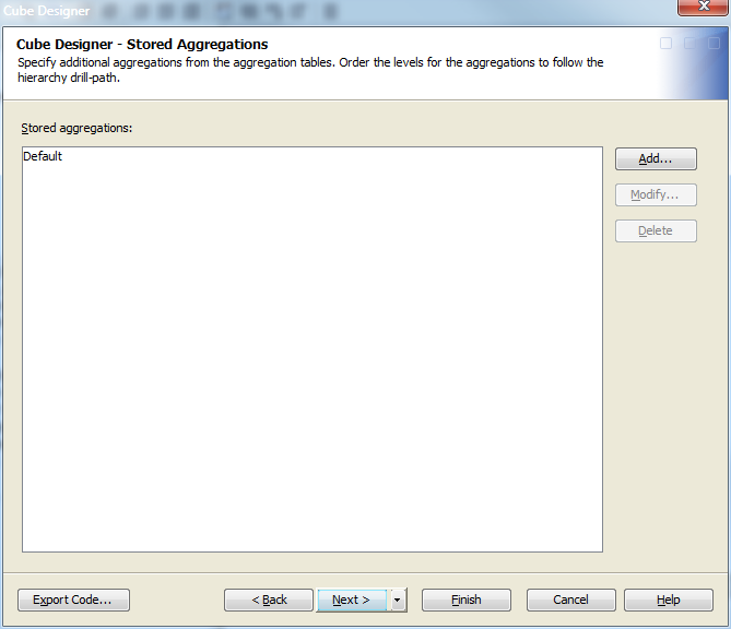
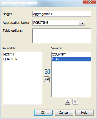
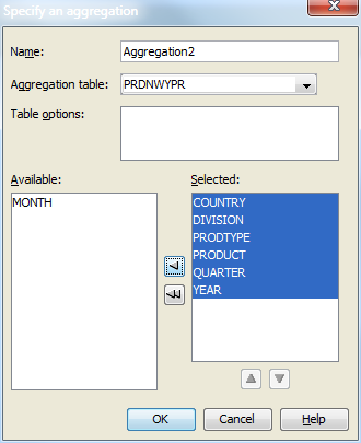
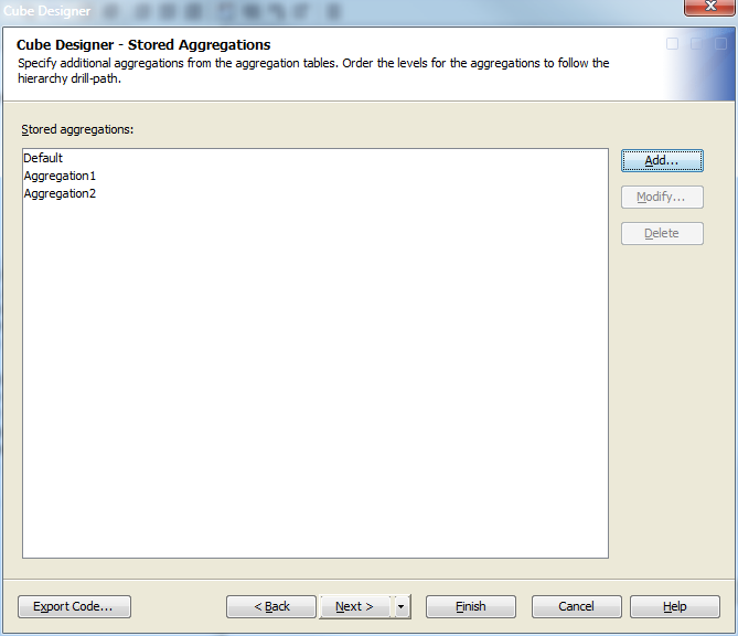
Define Stored Aggregations

You can now define stored aggregations for the cube. Stored aggregations are aggregations that are stored in the aggregation tables. On the Cube Designer - Stored Aggregations page, click Add to create a stored aggregation.

In the Specify an aggregation dialog box, enter the aggregation name, aggregation table, and any necessary table options for the aggregation. Then select the levels that are used in the aggregation. For this example, the stored aggregations named Aggregation1 and Aggregation2 are created.

The aggregations are listed on the Cube Designer – Stored Aggregations page.

Define Aggregations

If needed, you can now define aggregations that are stored with the cube. Define the aggregations for the cube from the Cube Designer – Aggregations page.

Build the Cube

After you have finished entering information for the summarized cube, you can build the cube. On the Finish page, you can review the details of the cube that you just defined, and then save your PROC OLAP code to a file and click Finish. The Finish dialog box is displayed as shown.

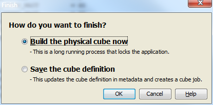
Select one of the cube creation options and click OK to save and build the cube.

PROC OLAP CODE for the Summary Table Example

OPTIONS VALIDVARNAME=ANY;
LIBNAME olapsio BASE  “\\olap\tmp\libolap" ;

PROC OLAP
   CUBE                   = "/Shared Data/OLAPSchemas/SumCube"
   PATH                   = 'C:\v9cubes'
   DESCRIPTION            = 'Fully Summarized Cube'
   NONUPDATEABLE
   MAXTHREADS             = 5000
;


   METASVR
      HOST        = "J12345.na.sas.com"
      PORT        = 8561
      OLAP_SCHEMA = "SASApp - OLAP Schema";

   DIMENSION Geography
      CAPTION          = 'Geography'
      SORT_ORDER       = ASCENDING
      HIERARCHIES      = (
         Geography
         ) /* HIERARCHIES */;

      HIERARCHY Geography
         ALL_MEMBER = 'All Geography'
         CAPTION    = 'Geography'
         LEVELS     = (
            COUNTRY DIVISION
            ) /* LEVELS */
         DEFAULT;

      LEVEL COUNTRY
         FORMAT         =  $CHAR10.
         CAPTION        =  'Country'
         SORT_ORDER     =  ASCENDING;

      LEVEL DIVISION
         FORMAT         =  $CHAR10.
         CAPTION        =  'Division'
         SORT_ORDER     =  ASCENDING;

   DIMENSION Products
      CAPTION          = 'Products'
      SORT_ORDER       = ASCENDING
      HIERARCHIES      = (
         Products
         ) /* HIERARCHIES */;

      HIERARCHY Products
         ALL_MEMBER = 'All Products'
         CAPTION    = 'Products'
         LEVELS     = (
            PRODUCT PRODTYPE
            ) /* LEVELS */
         DEFAULT;

      LEVEL PRODUCT
         FORMAT         =  $CHAR10.
         CAPTION        =  'Product'
         SORT_ORDER     =  ASCENDING;

      LEVEL PRODTYPE
         FORMAT         =  $CHAR10.
         CAPTION        =  'Product type'
         SORT_ORDER     =  ASCENDING;

   DIMENSION Dates
      CAPTION          = 'Dates'
      TYPE             = TIME
      SORT_ORDER       = ASCENDING
      HIERARCHIES      = (
         Dates
         ) /* HIERARCHIES */;

      HIERARCHY Dates
         ALL_MEMBER = 'All Dates'
         CAPTION    = 'Dates'
         LEVELS     = (
            YEAR QUARTER MONTH
            ) /* LEVELS */
         DEFAULT;

      LEVEL YEAR
         FORMAT         =  4.
         TYPE           =  YEAR
         CAPTION        =  'Year'
         SORT_ORDER     =  ASCENDING;

      LEVEL QUARTER
         FORMAT         =  8.
         TYPE           =  QUARTERS
         CAPTION        =  'Quarter'
         SORT_ORDER     =  ASCENDING;

      LEVEL MONTH
         FORMAT         =  MONNAME3.
         TYPE           =  MONTHS
         CAPTION        =  'Month'
         SORT_ORDER     =  ASCENDING;

   MEASURE predsumSUM
      STAT        = SUM
      ANALYSIS    = PredictGroup
      AGGR_COLUMN = predsum
      CAPTION     = 'Sum of predsum'
      FORMAT      = Best12.
      DEFAULT;

   MEASURE prednN
      STAT        = N
      ANALYSIS    = PredictGroup
      AGGR_COLUMN = predn
      CAPTION     = 'Number of values for predn'
      FORMAT      = 12.;

   MEASURE actsumSUM
      STAT        = SUM
      ANALYSIS    = ActualGroup
      AGGR_COLUMN = actsum
      CAPTION     = 'Sum of actsum'
      FORMAT      = Best12.;

   MEASURE actnN
      STAT        = N
      ANALYSIS    = ActualGroup
      AGGR_COLUMN = actn
      CAPTION     = 'Number of values for actn'
      FORMAT      = 12.;

   MEASURE PredictedDerived
      STAT        = AVG
      ANALYSIS    = PredictGroup
      CAPTION     = 'Average PredictGroup'
      FORMAT      = Best12.;

   MEASURE ActualDerived
      STAT        = AVG
      ANALYSIS    = ActualGroup
      CAPTION     = 'Average ActualGroup'
      FORMAT      = Best12.;

   AGGREGATION /* Default */
      /* levels */
      COUNTRY DIVISION MONTH PRODTYPE
      PRODUCT QUARTER YEAR
      / /* options */
      TABLE     = olapsio.PRDNWYPR
      NAME      = 'Default';

   AGGREGATION /* Aggregation1 */
      /* levels */
      COUNTRY YEAR
      / /* options */
      TABLE     = olapsio.PGEOTIME
      NAME      = 'Aggregation1';

   AGGREGATION /* Aggregation2 */
      /* levels */
      COUNTRY DIVISION PRODTYPE
      PRODUCT QUARTER YEAR
      / /* options */
      TABLE     = olapsio.PRDNWYPR
      NAME      = 'Aggregation2';

   RUN;

PROC OLAP Statements and Options for a Summary Table

The following table lists the PROC OLAP statements and options that you use to load cubes from a fully summarized data source. (A fully summarized data source contains a crossing of all dimensions. It is also known as an NWAY). Unlike a detail table or star schema, a fully summarized cube does not use either the DATA= or FACT= option. Instead, the TABLE= option is used in the AGGREGATION statement.

Statements and Options Used to Load Cubes from Fully Summarized Data

Statements	Options	Required or Optional
PROC OLAP	CUBE=	Required
	PATH=	Required
	DESC=	Optional
	NO_NWAY	Optional
	WORKPATH=	Optional
	DT_TABLE	Optional
METASVR	OLAP_SCHEMA=	Required
	REPOSITORY=	Optional
	HOST=	Optional
	PORT=	Optional
	PROTOCOL=	Optional
	USERID=	Optional
	PW=	Optional
DIMENSION	HIERARCHIES=	Required
	DESC=	Optional
	CAPTION=	Optional
	TYPE=TIME	Required only for TIME dimensions
	SORT_ORDER=	Optional
LEVEL		The LEVEL statement is optional unless you want to specify time periods for each level in a TIME dimension. If you specify a time period for one level, then you must specify a time period for all levels. To specify a time period, you use the TYPE= option.
HIERARCHY	LEVELS=	Required
	DESC=	Optional
	CAPTION=	Optional
MEASURE	STAT=	Required
	COLUMN \| ANALYSIS=	Required
	AGGR_COLUMN=	Required
	DESC=	Optional
	CAPTION=	Optional
	UNITS=	Optional
	FORMAT=	Optional
	DEFAULT=	Optional
PROPERTY	prop-name	Required
	LEVEL=	Required
AGGREGATION	Names of the contiguous levels to be used to create the aggregation	Required (additional AGGREGATION statements without the TABLE= option can be used to create aggregations other than the automatically defined NWAY).
	TABLE=	Required