Tutorial: A Module for Linear Regression

You can continue the example of this chapter by using the SCATTER subroutine to create scatter plots of the data, the predicted values, and the residuals.

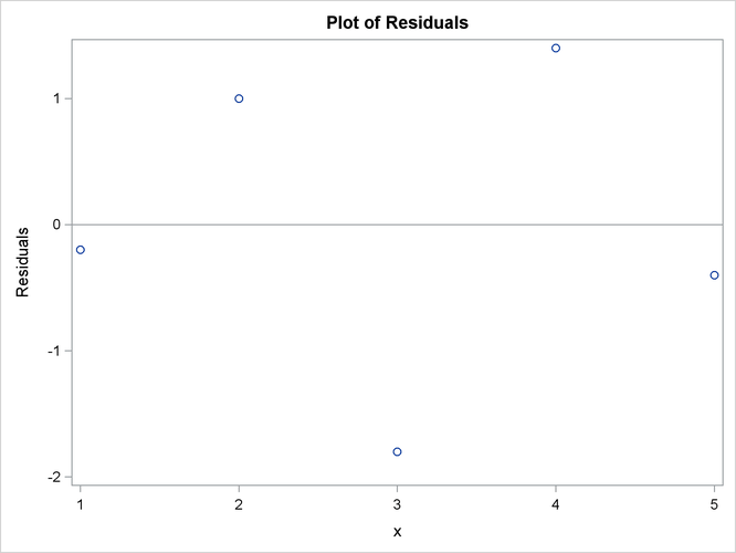
The following statements plot the residual values versus the explanatory variable. The graph is shown in Figure 4.8.

title "Plot of Residuals";
call scatter(x1, resid) label={"x" "Residuals"}
                        other="refline 0 / axis=y";

In a similar way, you can use the SCATTER routine to plot the predicted values against .

For more complicated graphs, you might choose to call the SGPLOT procedure directly from within your SAS/IML program. You can use the SUBMIT statement and ENDSUBMIT statement to call any SAS procedure from within PROC IML. For this example, you need to first create a SAS data set that contains the data. The following statements write the data to the RegData data set, then call the SGPLOT procedure to create a scatter plot overlaid with a line plot:

create RegData var {"x1" "y" "yhat"};
append;
close RegData;

submit;
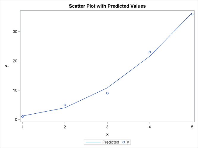
title "Scatter Plot with Predicted Values";
proc sgplot data=RegData;
   label x1="x" yhat="Predicted";
   series x=x1 y=yhat;
   scatter x=x1 y=y;
run;
endsubmit;

The CREATE statement creates a SAS data set named RegData. The APPEND statement writes the data to the data set. The SUBMIT and ENDSUBMIT statements bracket SAS programs statements that generate Figure 4.9.