CALL SPLINEC (fitted, coeff, endSlopes, data <*>, smooth <*>, delta <*>, nout <*>, type <*>, slope ) ;
The SPLINE and SPLINEC subroutines fit cubic splines to data. The SPLINE subroutine is the same as SPLINEC but does not return the matrix of spline coefficients needed to call SPLINEV, nor does it return the slopes at the endpoints of the curve.
The SPLINEC subroutine returns the following values:
- fitted
-
is an
 matrix of fitted values.
- coeff
-
is an
 (or
(or  ) matrix of spline coefficients. The matrix contains the cubic polynomial coefficients for the spline for each interval. Column
1 is the left endpoint of the
) matrix of spline coefficients. The matrix contains the cubic polynomial coefficients for the spline for each interval. Column
1 is the left endpoint of the  -interval for the regular (nonparametric) spline or the left endpoint of the parameter for the parametric spline. Columns
 are the constant, linear, quadratic, and cubic coefficients, respectively, for the -component. If a parametric spline is used, then columns
  are the constant, linear, quadratic, and cubic coefficients, respectively, for the
  -component. The coefficients for each interval are with respect to the variable
  where
where  is the left endpoint of the interval and is the point of interest. The matrix coeff can be processed to yield the integral or the derivative of the spline. This, in turn, can be used with the SPLINEV function
to evaluate the resulting curves. The SPLINEC subroutine returns coeff.
is the left endpoint of the interval and is the point of interest. The matrix coeff can be processed to yield the integral or the derivative of the spline. This, in turn, can be used with the SPLINEV function
to evaluate the resulting curves. The SPLINEC subroutine returns coeff.
- endSlopes
-
is a
 matrix that contains the slopes of the two ends of the curve expressed as angles in degrees. The SPLINEC subroutine returns
the endSlopes argument.
matrix that contains the slopes of the two ends of the curve expressed as angles in degrees. The SPLINEC subroutine returns
the endSlopes argument.
The input arguments to the SPLINEC subroutine are as follows:
- data
-
specifies a
(or  ) matrix of
  points on which the spline is to be fit. The optional third column is used to specify a weight for each data point. If smooth
  , the weight column is used in calculations. A weight
  causes the data point to be ignored in calculations.
- smooth
-
is an optional scalar that specifies the degree of smoothing to be used. If smooth is omitted or set equal to 0, then a cubic interpolating spline is fit to the data. If smooth
, then a cubic spline is used. Larger values of smooth generate more smoothing.
- delta
-
is an optional scalar that specifies the resolution constant. If delta is specified, the fitted points are spaced by the amount delta on the scale of the first column of data if a regular spline is used or on the scale of the curve length if a parametric spline is used. If both nout and delta are specified, nout is used and delta is ignored.
- nout
-
is an optional scalar that specifies the number of fitted points to be computed. The default is nout=200. If nout is specified, then nout equally spaced points are returned. The nout argument overrides the delta argument.
- type
-
is an optional
 (or ) character matrix or quoted literal that contains the type of spline to be used. The first element of type should be one of the following:
-
“periodic”, which requests periodic endpoints
-
“zero”, which sets second derivatives at endpoints to 0
The type argument controls the endpoint constraints unless the slope argument is specified. If “periodic” is specified, the response values at the beginning and end of column 2 of data must be the same unless the smoothing spline is being used. If the values are not the same, an error message is printed and no spline is fit. The default value is “zero”. The second element of type should be one of the following.
-
“nonparametric”, which requests a nonparametric spline
-
“parametric”, which requests a parametric spline
If “parametric” is specified, a parameter sequence
 is formed as follows:
  and
and
![\[ t_ i=t_{i-1} + \sqrt { (x_ i - x_{i-1})^2 + (y_ i - y_{i-1})^2 } \]](images/imlug_langref1421.png)
Splines are then fit to both the first and second columns of data. The resulting splined values are paired to form the output. Changing the relative scaling of the first two columns of data changes the output because the sequence
assumes Euclidean distance.
Note that if the points are not arranged in strictly ascending order by the first columns of data, then a parametric method must be used. An error message results if the nonparametric spline is requested.
-
- slope
-
is an optional
matrix of endpoint slopes given as angles in degrees. If a parametric spline is used, the angle values are used modulo 360.
If a nonparametric spline is used, the tangent of the angles is used to set the slopes (that is, the effective angles range
from  to
to  degrees).
See Stoer and Bulirsch (1980), Reinsch (1967), and Pizer (1975) for descriptions of the methods used to fit the spline. For simplicity, the following explanation assumes that the data matrix does not contain a weighting column.
Nonparametric splines can be used to fit data for which you believe there is a functional relationship between the X and Y
variables. The unique values of X (stored in the first column of data) form a partition ![]() of the interval
of the interval ![]() . You can use a spline to interpolate the data (produce a curve that passes through each data point) provided that there is
a single Y value for each X value. The spline is created by constructing cubic polynomials on each subinterval
. You can use a spline to interpolate the data (produce a curve that passes through each data point) provided that there is
a single Y value for each X value. The spline is created by constructing cubic polynomials on each subinterval ![]() so that the value of the cubic polynomials and their first two derivatives coincide at each
so that the value of the cubic polynomials and their first two derivatives coincide at each ![]() .
.
An interpolating spline is not uniquely determined by the set of Y values. To achieve a unique interpolant, ![]() , you must specify two constraints on the endpoints of the interval
, you must specify two constraints on the endpoints of the interval ![]() . You can achieve uniqueness by specifying one of the following conditions:
. You can achieve uniqueness by specifying one of the following conditions:
-
 The second derivative at both endpoints is zero. This is the default condition, but can be explicitly set by using
 type=’zero’. -
Periodic conditions. If your data are periodic so that
 can be identified with
  , and if
  , then the interpolating spline already satisfies
  . Setting
 type=’periodic’further requires that and
and  .
.
-
Fixed slopes at endpoints. Setting slope=
 requires that
  and
and  .
.
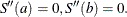
The following statements give three examples of computing an interpolating spline for data. Note that the first and last Y values are the same, so you can ask for a periodic spline.
proc iml;
data = { 0 5, 1 3, 2 5, 3 4, 4 6, 5 7, 6 6, 7 5 };

/* Compute three spline interpolants of the data */
/* (1) a cubic spline with type=zero (the default) */
call spline(fitted,data);

/* (2) A periodic spline */
call spline(periodicFitted,data) type='periodic';

/* (3) A spline with specific slopes at endpoints */
call spline(slopeFitted,data) slope={45 30};

/* write data */
create SplineData from data[colname={"x" "y"}];
append from data;
close SplineData;

/* write fitted interpolants */
fit = fitted || periodicFitted[,2] || slopeFitted[,2];
varNames = {"t" "Interpolant" "Periodic" "EndSlopes"};
create SplineFit from fit[colname=varNames];
append from fit;
close SplineFit;
quit;

/* merge data and plot */
data Spline;
merge SplineData SplineFit;
run;

title "Spline Interpolation";
proc sgplot data=Spline;
   scatter x=x y=y;
   series x=t y=Interpolant;
   series x=t y=Periodic / lineattrs=(color="dark red");
   series x=t y=EndSlopes / lineattrs=(color="dark green");
run;
As shown in Figure 24.379, the interpolants pass through each point of the data. They differ from each other by the derivatives at the boundary points,
![]() and
and ![]() . The generic interpolant has second derivatives that vanish at the boundary points. The periodic curve has a derivative at
. The generic interpolant has second derivatives that vanish at the boundary points. The periodic curve has a derivative at
![]() that matches the derivative at
that matches the derivative at ![]() . The third curve has derivatives that match the given slopes at the boundary points.
. The third curve has derivatives that match the given slopes at the boundary points.
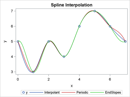
You can also use a spline to smooth data. In general, a smoothing spline does not pass through any data pair exactly. A very small value of the smooth smoothing parameter approximates an interpolating polynomial for data in which each unique X value is assigned the mean of the Y values that correspond to that X value. As the smooth parameter gets very large, the spline approximates a linear regression.
The following statements compute two smoothing splines for the same data as in the previous example. The spline coefficients are passed to the SPLINEV function, which evaluates the smoothing spline at the original X values. The smoothing spline does not pass through the original Y values. Also, the smoothing parameter for the periodic spline is smaller, so the periodic spline has more “wiggles” than the corresponding spline with the larger smoothing parameter.
proc iml;
data = { 0 5, 1 3, 2 5, 3 4, 4 6, 5 7, 6 6, 7 5 };

/* Compute spline smoothers of the data. */
call splinec(fitted,coeff,endSlopes,data) smooth=1;

/* Evaluate the smoother at the original X positions */
smoothFit = splinev(coeff, data[,1]);

/* Compute periodic spline smoother of the data. */
call splinec(periodicFitted,coeff,endSlopesP,data)
             smooth=0.1 type="periodic";

/* Evaluate the smoother at the original X positions */
smoothPeriodicFit = splinev(coeff, data[,1]);

/* Compare the two fits */
print smoothFit smoothPeriodicFit;
Figure 24.380: Two Spline Smoothers
| smoothFit | smoothPeriodicFit | ||
|---|---|---|---|
| 0 | 4.4761214 | 0 | 4.7536432 |
| 1 | 4.002489 | 1 | 3.5603915 |
| 2 | 4.2424509 | 2 | 4.3820561 |
| 3 | 4.8254655 | 3 | 4.47148 |
| 4 | 5.7817386 | 4 | 5.8811872 |
| 5 | 6.3661254 | 5 | 6.8331581 |
| 6 | 6.0606327 | 6 | 6.1180839 |
| 7 | 5.2449764 | 7 | 4.7536432 |
You can write the smoothers to a SAS data set and merge them with the data, as shown in the previous example. Figure 24.381 shows the resulting graph.
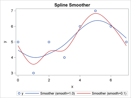
A parametric spline can be used to interpolate or smooth data for which there does not seem to be a functional relationship
between the X and Y variables. A partition ![]() is formed as explained in the documentation for the type parameter. Splines are then used to fit the X and Y values independently.
is formed as explained in the documentation for the type parameter. Splines are then used to fit the X and Y values independently.
The following program fits a parametric curve to data that are shaped like an “S.” The variable fitted is returned as a numParam ![]() matrix that contains the ordered pairs that correspond to the parametric spline. These ordered pairs correspond to numParam evenly spaced points in the domain of the parameter
matrix that contains the ordered pairs that correspond to the parametric spline. These ordered pairs correspond to numParam evenly spaced points in the domain of the parameter ![]() .
.
The purpose of the SPLINEV function is to evaluate (score) an interpolating or smoothing spline at an arbitrary set of points. The following program shows how to construct the parameters that correspond to the original data by using the formula specified in the documentation for the type argument. These parameters are used to construct the evenly spaced parameters that correspond to the data in the fitted matrix.
proc iml;
data = {3 7, 2 7, 1 6, 1 5, 2 4, 3 3, 3 2, 2 1, 1 1};

/* Compute parametric spline interpolant */
numParam = 40;
call splinec(fitted,coeff,endSlopes,data)
             nout=numParam type={"zero" "parametric"};

/* write data */
create SplineData from data[colname={"x" "y"}];
append from data;
close SplineData;

/* write parametric spline values */
create SplineFit from fitted[colname={"xt" "yt"}];
append from fitted;
close SplineFit;


/* Manually reproduce/verify the "fitted" values */
/* (1) Form the parameters mapped onto the data */
t = j(nrow(data),1,0); /* first parameter is zero */
do i = 2 to nrow(t);
   t[i] = t[i-1] + sqrt( (data[i,1]-data[i-1,1])##2 +
                         (data[i,2]-data[i-1,2])##2 );
end;

/* (2) Construct numParam evenly spaced parameters
   between 0 and t[nrow(t)] */
params = do(0, t[nrow(t)], t[nrow(t)]/(numParam-1))`;

/* (3) Evaluate the parametric spline at these points */
fit = splinev(coeff, params);
maxDiff = max(abs(fitted-fit));
print maxDiff; /* should be very small or zero */
quit;

/* merge data and plot */
data Spline;
merge SplineData SplineFit;
run;

title "Parametric Spline Smoother";
proc sgplot data=Spline;
   scatter x=x y=y;
   series x=xt y=yt / legendlabel="Parametric Spline";
run;
Attempting to evaluate a spline outside its domain of definition results in a missing value. For example, the following statements
define a spline on the interval ![]() . Attempting to evaluate the spline at points outside this interval (
. Attempting to evaluate the spline at points outside this interval (![]() or
or ![]() ) results in missing values.
) results in missing values.
proc iml;
data = { 0 5, 1 3, 2 5, 3 4, 4 6, 5 7, 6 6, 7 5 };
call splinec(fitted,coeff,endSlopes,data) slope={45 45};
v =  splinev(coeff,{-1 1 2 3 3.5 4 20});
print v;
One use of splines is to estimate the integral of a function that is known only by its value at a discrete set of points. Many people are familiar with elementary methods of numerical integration such as the left-hand rule, the trapezoid rule, and Simpson’s rule. In the left-hand rule, the integral of discrete data is estimated by the exact integral of a piecewise constant function between the data points. In the trapezoid rule, the integral is estimated by the exact integral of a piecewise linear function that connects the data points. In Simpson’s rule, the integral is estimated as the exact integral of a piecewise quadratic function between the data points.
Because a cubic spline is a sequence of cubic polynomials, it is possible to compute the exact integral of the cubic spline and use this as an estimate for the integral of the discrete data. The next example takes a function defined by discrete data and finds the integral and the first moment of the function.
The implementation of the integrand function (SpleinEval) uses a helpful trick to evaluate a spline at a single point. If you pass in a scalar argument to the SPLINEV function, you
get back a vector that represents the evaluation of the spline along evenly spaced points, rather than the spline evaluated
at the argument. To avoid this, the following statements evaluate the spline at the vector x // x and then extract the entry in the first row, second column. This number is the value of the spline evaluated at ![]() .
.
proc iml;
x = { 0, 2, 5, 7, 8, 10 };
y = x + 0.1*sin(x);
a = x || y;
call splinec(fit,coeff,endSlopes,a);

start SplineEval(x) global(coeff,power);
   /* The first column of v contains the points of evaluation;
      the second column contains the evaluation. */
   v = x##power # splinev(coeff, x//x);
   return(v[1,2]); /* return spline(x) */
finish;

/* Evaluate the "moment" of a function.
   moment(0) = integral of f(x) dx
   moment(1) = integral of x*f(x) dx
   moment(2) = integral of x##2 *f(x) dx, etc
   Use QUAD to integrate */
start moment(pow) global(coeff,power);
   power = pow;
   intervals = coeff[,1]; /* left endpts of x intervals */
   call quad(z,"SplineEval", intervals) eps = 1.e-10;
   return( sum(z) );
finish;

mass  = moment(0);   /* to compute the mass */
m     = mass //
       (moment(1)/mass) // /* to compute the mean */
       (moment(2)/mass) ;  /* to compute the meansquare */
print m;


/* Check the previous computation by using Gauss-Legendre
   integration, which is valid for moments up to maxng. */
gauss = {
    -9.3246951420315205e-01      -6.6120938646626448e-01
    -2.3861918608319743e-01       2.3861918608319713e-01
     6.6120938646626459e-01       9.3246951420315183e-01,
     1.713244923791701e-01        3.607615730481388e-01
     4.679139345726905e-01        4.679139345726904e-01
     3.607615730481389e-01        1.713244923791707e-01  };
ngauss = ncol(gauss); /* = 6 */
maxng  =  2*ngauss-4;

start momentGL(pow) global(coeff,gauss,ngauss,maxng);
   if pow >= maxng  then return(.);
   nrow    = nrow(coeff);
   left    = coeff[1:nrow-1,1]; /* left endpt of interval */
   right   = coeff[2:nrow,1];   /* right endpt */
   mid     = 0.5*(left+right);
   interv  = 0.5*(right - left);
   /* scale the weights on each interval */
   wgts    = rowvec( interv*gauss[2,] );
   /* scale the points on each interval */
   pts     = rowvec( interv*gauss[1,] + mid );
   /* evaluate the function */
   eval    = splinev(coeff,pts)[,2]`;
   return( sum( wgts#pts##pow # eval) );
finish;

mass  = momentGL(0);       /* to compute the mass */
m2    = mass // (momentGL(1)/mass) //  (momentGL(2)/mass) ;
print m2; /* should agree with earlier result */
Figure 24.385: Integral and Other Moments of the Spline Function
| m |
|---|
| 50.204224 |
| 6.658133 |
| 49.953307 |
| m2 |
|---|
| 50.204224 |
| 6.658133 |
| 49.953307 |