Nonlinear Optimization Examples

Example 11.8: Time-Optimal Heat Conduction

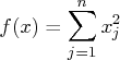
The following example illustrates a nontrivial application of the NLPQN algorithm that requires nonlinear constraints, which are specified by the nlc module. The example is listed as problem 91 in Hock and Schittkowski (1981). The problem describes a time-optimal heating process minimizing the simple objective function

subjected to a rather difficult inequality constraint:

where is defined as

The gradient of the objective function , , is easily supplied to the NLPQN subroutine. However, the analytical derivatives of the constraint are not used; instead, finite-difference derivatives are computed.

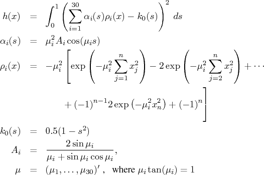
In the following code, the vector MU represents the first 30 positive values that satisfy :

  
    proc iml; 
       mu = { 8.6033358901938E-01 ,    3.4256184594817E+00 , 
              6.4372981791719E+00 ,    9.5293344053619E+00 , 
              1.2645287223856E+01 ,    1.5771284874815E+01 , 
              1.8902409956860E+01 ,    2.2036496727938E+01 , 
              2.5172446326646E+01 ,    2.8309642854452E+01 , 
              3.1447714637546E+01 ,    3.4586424215288E+01 , 
              3.7725612827776E+01 ,    4.0865170330488E+01 , 
              4.4005017920830E+01 ,    4.7145097736761E+01 , 
              5.0285366337773E+01 ,    5.3425790477394E+01 , 
              5.6566344279821E+01 ,    5.9707007305335E+01 , 
              6.2847763194454E+01 ,    6.5988598698490E+01 , 
              6.9129502973895E+01 ,    7.2270467060309E+01 , 
              7.5411483488848E+01 ,    7.8552545984243E+01 , 
              8.1693649235601E+01 ,    8.4834788718042E+01 , 
              8.7975960552493E+01 ,    9.1117161394464E+01  };
 

The vector depends only on and is computed only once, before the optimization starts, as follows:

  
    nmu  = nrow(mu); 
    a = j(1,nmu,0.); 
    do i = 1 to nmu; 
       a[i] = 2*sin(mu[i]) / (mu[i] + sin(mu[i])*cos(mu[i])); 
    end;
 

The constraint is implemented with the QUAD subroutine, which performs numerical integration of scalar functions in one dimension. The subroutine calls the module fquad that supplies the integrand for . For details about the QUAD call, see the section "QUAD Call". Here is the code:

  
   /* This is the integrand used in h(x) */ 
    start fquad(s) global(mu,rho); 
       z = (rho * cos(s*mu) - 0.5*(1. - s##2))##2; 
       return(z); 
    finish; 
  
   /* Obtain nonlinear constraint h(x) */ 
    start h(x) global(n,nmu,mu,a,rho); 
       xx = x##2; 
       do i= n-1 to 1 by -1; 
          xx[i] = xx[i+1] + xx[i]; 
       end; 
       rho = j(1,nmu,0.); 
       do i=1 to nmu; 
          mu2 = mu[i]##2; 
          sum = 0; t1n = -1.; 
          do j=2 to n; 
             t1n = -t1n; 
             sum = sum + t1n * exp(-mu2*xx[j]); 
          end; 
          sum = -2*sum + exp(-mu2*xx[1]) + t1n; 
          rho[i] = -a[i] * sum; 
       end; 
       aint = do(0,1,.5); 
       call quad(z,"fquad",aint) eps=1.e-10; 
       v = sum(z); 
       return(v); 
    finish;
 

The modules for the objective function, its gradient, and the constraint are given in the following code:

  
   /* Define modules for NLPQN call: f, g, and c */ 
    start F_HS88(x); 
       f = x * x`; 
       return(f); 
    finish F_HS88; 
  
    start G_HS88(x); 
       g = 2 * x; 
       return(g); 
    finish G_HS88; 
  
    start C_HS88(x); 
       c = 1.e-4 - h(x); 
       return(c); 
    finish C_HS88;
 

The number of constraints returned by the "nlc" module is defined by opt. The ABSGTOL termination criterion (maximum absolute value of the gradient of the Lagrange function) is set by tcE-4. Here is the code:

  
    print 'Hock & Schittkowski Problem #91 (1981) n=5, INSTEP=1'; 
    opt  = j(1,10,.); 
    opt[2]=3; 
    opt[10]=1; 
    tc   = j(1,12,.); 
    tc[6]=1.e-4; 
    x0 = {.5 .5 .5 .5 .5}; 
    n = ncol(x0); 
    call nlpqn(rc,rx,"F_HS88",x0,opt,,tc) grd="G_HS88" nlc="C_HS88";
 

Part of the iteration history and the parameter estimates are shown in Output 11.8.1.

Output 11.8.1: Iteration History and Parameter Estimates

---

Dual Quasi-Newton Optimization

Modified VMCWD Algorithm of Powell (1978, 1982)

Dual Broyden - Fletcher - Goldfarb - Shanno Update (DBFGS)

Lagrange Multiplier Update of Powell(1982)

Jacobian Nonlinear Constraints Computed by Finite Differences

Parameter Estimates	5
Nonlinear Constraints	1

Optimization Start
Objective Function	1.25	Maximum Constraint Violation	0.0952775105
Maximum Gradient of the Lagran Func	1.1433393624

Iteration		Restarts	Function Calls	Objective Function	Maximum Constraint Violation	Predicted Function Reduction	Step Size	Maximum Gradient Element of the Lagrange Function
1		0	3	0.81165	0.0869	1.7562	0.100	1.325
2		0	4	0.18232	0.1175	0.6220	1.000	1.207
3	*	0	5	0.34567	0.0690	0.9321	1.000	0.639
4		0	6	0.77699	0.0132	0.3498	1.000	1.329
.	.	.	.	.	.	.	.	.
.	.	.	.	.	.	.	.	.
.	.	.	.	.	.	.	.	.
21		0	30	1.36266	8.06E-12	1.075E-6	1.000	0.00009

Optimization Results
Iterations	21	Function Calls	31
Gradient Calls	23	Active Constraints	1
Objective Function	1.3626568064	Maximum Constraint Violation	8.05972E-12
Maximum Projected Gradient	0.0000966554	Value Lagrange Function	1.3626568149
Maximum Gradient of the Lagran Func	0.0000889516	Slope of Search Direction	-1.074804E-6

ABSGCONV convergence criterion satisfied.

---

Optimization Results
Parameter Estimates
N	Parameter	Estimate	Gradient Objective Function	Gradient Lagrange Function
1	X1	0.860296	1.720591	0.000031041
2	X2	0.000002240	0.000004481	0.000015290
3	X3	0.643469	1.286938	0.000021632
4	X4	0.456614	0.913227	-0.000088952
5	X5	0.000000905	0.000001811	0.000077582

Value of Objective Function = 1.3626568064

Value of Lagrange Function = 1.3626568149

Problems 88 to 92 of Hock and Schittkowski (1981) specify the same optimization problem for to . You can solve any of these problems with the preceding code by submitting a vector of length as the initial estimate, .