| Language Reference |
FARMACOV Call
computes the autocovariance function for
an ARFIMA(![]() ) process
) process
- CALL FARMACOV( cov, d <, phi, theta, sigma, p, q, lag>);
The inputs to the FARMACOV subroutine are as follows:
- d
- specifies a fractional differencing order.
The value of
 must be in the open interval
  excluding zero.
This input is required.
excluding zero.
This input is required.
- phi
- specifies an
 -dimensional vector
containing the autoregressive coefficients,
where is the number of the elements in the subset
of the AR order. The default is zero.
All the roots of
-dimensional vector
containing the autoregressive coefficients,
where is the number of the elements in the subset
of the AR order. The default is zero.
All the roots of  should be greater than one
in absolute value,
where
should be greater than one
in absolute value,
where  is the finite-order matrix polynomial in the backshift
operator
is the finite-order matrix polynomial in the backshift
operator  , such that
  .
. - theta
- specifies an
 -dimensional vector
containing the moving-average coefficients,
where is the number of the elements in the subset
of the MA order. The default is zero.
-dimensional vector
containing the moving-average coefficients,
where is the number of the elements in the subset
of the MA order. The default is zero.
- p
- specifies the subset of the AR order. The quantity is defined as
the number of elements of phi.
If you do not specify p, the default subset is p .
.
For example, consider phi=0.5.
If you specify p=1 (the default), the FARMACOV subroutine computes the theoretical autocovariance function of an ARFIMA( ) process as
If you specify p=2, the FARMACOV subroutine computes the autocovariance function of an ARFIMA( ) process as
- q
- specifies the subset of the MA order. The quantity is defined as
the number of elements of theta.
If you do not specify q, the default subset is q .
.
The usage of q is the same as that of p. - lag
- specifies the length of lags, which must be a positive number.
The default is
 .
.
The FARMACOV subroutine returns the following value:
- cov
- is a
 vector containing
the autocovariance function of an ARFIMA(
vector containing
the autocovariance function of an ARFIMA( ) process.
Consider the following ARFIMA(
    d    = 0.3;
    phi  = 0.5;
    theta= -0.1;
    sigma= 1.2;
    call farmacov(cov, d, phi, theta, sigma) lag=5;
    print cov;
For
The FARMACOV subroutine computes the autocovariance function of an ARFIMA(
For
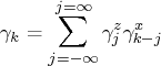
Let
Then the autocovariance function of
Copyright © 2009 by SAS Institute Inc., Cary, NC, USA. All rights reserved.