Language Reference: EIGEN Call :: SAS/IML(R) 9.2 User's Guide

Language Reference

EIGEN Call

computes eigenvalues and eigenvectors

CALL EIGEN( eigenvalues, eigenvectors, ) <VECL="vl">;

where

is an arbitrary square numeric matrix for which eigenvalues and eigenvectors are to be calculated.

The EIGEN call returns the following values:

eigenvalues: a matrix to contain the eigenvalues of the input matrix.
eigenvectors: names a matrix to contain the right eigenvectors of the input matrix.
vl: is an optional matrix containing the left eigenvectors of in the same manner that eigenvectors contains the right eigenvectors.

The EIGEN subroutine computes eigenvalues, a matrix containing the eigenvalues of

. If

is symmetric, eigenvalues is the

vector containing the

real eigenvalues of

. If

is not symmetric (as determined by the criteria in the symmetry test described later), eigenvalues is an

matrix containing the eigenvalues of the

matrix

. The first column of

contains the real parts, ${re}(\lambda)$ , and the second column contains the imaginary parts ${im}(\lambda)$ . Each row represents one eigenvalue, ${re}(\lambda) + i{im}(\lambda)$ .

If

is symmetric, the eigenvalues are arranged in descending order. Otherwise, the eigenvalues are sorted first by their real parts, then by the magnitude of their imaginary parts. Complex conjugate eigenvalues, ${re}(\lambda)+- i{im}(\lambda)$ , are stored in standard order; that is, the eigenvalue of the pair with a positive imaginary part is followed by the eigenvalue of the pair with the negative imaginary part.

The EIGEN subroutine also computes eigenvectors, a matrix. If

is symmetric, then eigenvectors has orthonormal column eigenvectors of

arranged so that the matrices correspond; that is, the first column of eigenvectors is the eigenvector corresponding to the largest eigenvalue, and so forth. If

is not symmetric, then eigenvectors is an

matrix containing the right eigenvectors of

. If the eigenvalue in row

of eigenvalues is real, then column

of eigenvectors contains the corresponding real eigenvector. If rows

and

of eigenvalues contain complex conjugate eigenvalues ${re}(\lambda)+- i{im}(\lambda)$ , then columns

and

of eigenvectors contain the real,

, and imaginary,

, parts, respectively, of the two corresponding eigenvectors

.

The eigenvalues of a matrix

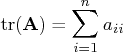
are the roots of the characteristic polynomial, which is defined as $p(z) = \det(z{i}- {a})$ . The spectrum, denoted by $\lambda(a)$ , is the set of eigenvalues of the matrix

. If $\lambda({a})=\{\lambda_1, ... ,\lambda_n\}$ , then $\det({a}) = \lambda_1 \lambda_2 ... \lambda_n$ .

The trace of

is defined by

${\rm tr}({a}) = \sum_{i=1}^n a_{ii}$

and tr $({a})= \lambda_1 + ... + \lambda_n$ .

An eigenvector is a nonzero vector,

, that satisfies ${a}{x}= \lambda{x}$ for $\lambda \in \lambda({a})$ . Right eigenvectors satisfy ${a}{x}= \lambda{x}$ , and left eigenvectors satisfy ${x}^h{a}= \lambda{x}^h$ , where ${x}^h$ is the complex conjugate transpose of

. Taking the conjugate transpose of both sides shows that left eigenvectors also satisfy ${a}^'{x}= \bar{\lambda}{x}$ .

The following are properties of the unsymmetric real eigenvalue problem, in which the real matrix

is square but not necessarily symmetric:

The eigenvalues of an unsymmetric matrix can be complex. If has a complex eigenvalue 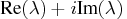${re}(\lambda) + i{im}(\lambda)$ , then the conjugate complex value ${re}(\lambda)-i{im}(\lambda)$ is also an eigenvalue of .
The right and left eigenvectors corresponding to a real eigenvalue of are real. The right and left eigenvectors corresponding to conjugate complex eigenvalues of are also conjugate complex.
The left eigenvectors of are the same as the complex conjugate right eigenvectors of ${a}^'$ .

The three routines, EIGEN, EIGVAL, and EIGVEC, use the following test of symmetry for a square argument matrix

Select the entry of with the largest magnitude:
$a_{max} = \max_{i,j=1, ... ,n} | a_{i,j}|$
Multiply the value of $a_{max}$ by the square root of the machine precision $\epsilon$ . (The value of $\epsilon$ is the largest value stored in double precision that, when added to 1 in double precision, still results in 1.)
The matrix is considered unsymmetric if there exists at least one pair of symmetric entries that differs in more than $a_{max}\sqrt{\epsilon}$ ,
$| a_{i,j}-a_{j,i}| \gt a_{max} \sqrt{\epsilon}$

Consider the following statement:

  
    call eigen(m,e,a);

is symmetric, then the output of this statement has the following properties:

$a*e & = & e*{diag}(m) \ e^'*e & = & i(n)$

These properties imply the following:

$e^' = {inv}(e)$

$a = e*{diag}(m)*e^'$

The QL method is used to compute the eigenvalues (Wilkinson and Reinsch 1971).

In statistical applications, nonsymmetric matrices for which eigenvalues are desired are usually of the form $e^{-1} h$ , where and are symmetric. The eigenvalues and eigenvectors of $e^{-1} h$ can be obtained by using the GENEIG subroutine or as follows:

  
    f=root(einv); 
    a=f*h*f'; 
    call eigen(l,w,a); 
    v=f'*w;

The computation can be checked by forming the residuals. Here is the code:

  
    r=einv*h*v-v*diag(l);

The values in

should be of the order of rounding error.

The following code computes the eigenvalues and left and right eigenvectors of a nonsymmetric matrix with four real and four complex eigenvalues:

  
    A = {-1  2  0       0       0       0       0  0, 
         -2 -1  0       0       0       0       0  0, 
          0  0  0.2379  0.5145  0.1201  0.1275  0  0, 
          0  0  0.1943  0.4954  0.1230  0.1873  0  0, 
          0  0  0.1827  0.4955  0.1350  0.1868  0  0, 
          0  0  0.1084  0.4218  0.1045  0.3653  0  0, 
          0  0  0       0       0       0       2  2, 
          0  0  0       0       0       0      -2  0 }; 
    call eigen(val,rvec,A) levec='lvec';

The sorted eigenvalues of this matrix are as follows:

  
                   VAL 
  
                   1 1.7320508 
                   1 -1.732051 
                   1         0 
           0.2087788         0 
           0.0222025         0 
           0.0026187         0 
                  -1         2 
                  -1        -2

You can verify the correctness of the left and right eigenvector computation by using the following code:

  
    /* verify right eigenvectors are correct */ 
    vec = rvec; 
    do j = 1 to ncol(vec); 
      /* if eigenvalue is real */ 
      if val[j,2] = 0. then do; 
        v = a * vec[,j] - val[j,1] * vec[,j]; 
        if any( abs(v) > 1e-12 ) then 
          badVectors = badVectors || j; 
        end; 
      /* if eigenvalue is complex with positive imaginary part */ 
      else if val[j,2] > 0. then do; 
        /* the real part */ 
        rp = val[j,1] * vec[,j] - val[j,2] * vec[,j+1]; 
        v = a * vec[,j] - rp; 
        /* the imaginary part */ 
        ip = val[j,1] * vec[,j+1] + val[j,2] * vec[,j]; 
        u = a * vec[,j+1] - ip; 
        if any( abs(u) > 1e-12 ) | any( abs(v) > 1e-12 ) then 
          badVectors = badVectors || j || j+1; 
        end; 
      end; 
    if ncol( badVectors ) > 0 then 
      print "Incorrect right eigenvectors:" badVectors; 
    else print "All right eigenvectors are correct";

Similar code can be written to verify the left eigenvectors, using the fact that the left eigenvectors of are the same as the complex conjugate right eigenvectors of ${a}^'$ . Here is the code:

  
    /* verify left eigenvectors are correct */ 
    vec = lvec; 
    do j = 1 to ncol(vec); 
      /* if eigenvalue is real */ 
      if val[j,2] = 0. then do; 
        v = a` * vec[,j] - val[j,1] * vec[,j]; 
        if any( abs(v) > 1e-12 ) then 
          badVectors = badVectors || j; 
        end; 
      /* if eigenvalue is complex with positive imaginary part */ 
      else if val[j,2] > 0. then do; 
        /* Note the use of complex conjugation */ 
        /* the real part */ 
        rp = val[j,1] * vec[,j] + val[j,2] * vec[,j+1]; 
        v = a` * vec[,j] - rp; 
        /* the imaginary part */ 
        ip = val[j,1] * vec[,j+1] - val[j,2] * vec[,j]; 
        u = a` * vec[,j+1] - ip; 
        if any( abs(u) > 1e-12 ) | any( abs(v) > 1e-12 ) then 
          badVectors = badVectors || j || j+1; 
        end; 
      end; 
    if ncol( badVectors ) > 0 then 
      print "Incorrect left eigenvectors:" badVectors; 
    else print "All left eigenvectors are correct";

The EIGEN call performs most of its computations in the memory allocated for returning the eigenvectors.

Top of Page