| Language Reference |
LMS Call
performs robust regression
- CALL LMS( sc, coef, wgt, opt,
 ,
,  ,
sorb>);
,
sorb>);
The Least Median of Squares (LMS) performs robust regression (sometimes called resistant regression) by minimizing the
The algorithm used in the LMS subroutine is based on the PROGRESS program of Rousseeuw and Hubert (1996), which is an updated version of Rousseeuw and Leroy (1987). In the special case of regression through the origin with a single regressor, Barreto and Maharry (2006) show that the PROGRESS algorithm does not, in general, find the slope that yields the least median of squares. Starting with release 9.2, the LMS subroutine uses the algorithm of Barreto and Maharry (2006) to obtain the correct LMS slope in the case of regression through the origin with a single regressor. In this case, inputs to the LMS subroutine specific to the PROGRESS algorithm are ignored and output specific to the PROGRESS algorithm is suppressed.
The value of
In the following discussion,
- opt
- refers to an options vector with the following components
(missing values are treated as default values).
The options vector can be a null vector.
- opt[1]
- specifies whether an intercept is used in the model
(opt[1]=0) or not (opt[1]
 ).
If opt[1]=0, then a column of ones is added as
the last column to the input matrix
).
If opt[1]=0, then a column of ones is added as
the last column to the input matrix  ; that
is, you do not need to add this column of ones yourself.
The default is opt[1]=0.
; that
is, you do not need to add this column of ones yourself.
The default is opt[1]=0.
- opt[2]
- specifies the amount of printed output.
Higher values request additional output
and include the output of lower values.
- opt[2]=0
- prints no output except error messages.
- opt[2]=1
- prints all output except (1) arrays of
 ,
such as weights, residuals, and diagnostics; (2)
the history of the optimization process; and (3)
subsets that result in singular linear systems.
,
such as weights, residuals, and diagnostics; (2)
the history of the optimization process; and (3)
subsets that result in singular linear systems.
- opt[2]=2
- additionally prints arrays of , such
as weights, residuals, and diagnostics;
also prints the case numbers of the
observations in the best subset and some
basic history of the optimization process.
- opt[2]=3
- additionally prints subsets that result in singular linear systems.
The default is opt[2]=0.
- opt[3]
- specifies whether only LMS is computed or
whether, additionally, least squares (LS) and
weighted least squares (WLS) regression are computed.
- opt[3]=0
- computes only LMS.
- opt[3]=1
- computes, in addition to LMS, weighted
least squares regression on the observations
with small LMS residuals (where
small is defined by opt[8]).
- opt[3]=2
- computes, in addition to LMS,
unweighted least squares regression.
- opt[3]=3
- adds both unweighted and weighted least squares regression to LMS regression.
The default is opt[3]=0.
- opt[4]
- specifies the quantile
 to be minimized.
This is used in the objective function.
The default is opt[4]
to be minimized.
This is used in the objective function.
The default is opt[4]![=h=[\frac{n+n+1}2]](images/langref_langrefeq688.gif) , which
corresponds to the highest possible breakdown value.
This is also the default of the PROGRESS program.
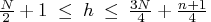
The value of should be in the range
, which
corresponds to the highest possible breakdown value.
This is also the default of the PROGRESS program.
The value of should be in the range
- opt[5]
- specifies the number
 of generated subsets.
Each subset consists of
of generated subsets.
Each subset consists of  observations
 , where
  .
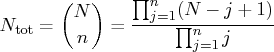
The total number of subsets consisting of
observations out of
.
The total number of subsets consisting of
observations out of  observations is
is the number of
parameters including the intercept.
observations is
is the number of
parameters including the intercept.
Due to computer time restrictions, not all subset combinations of observations out of can
be inspected for larger values of and .
Specifying a value of  enables you to save computer time at the
expense of computing a suboptimal solution.
enables you to save computer time at the
expense of computing a suboptimal solution.
If opt[5] is zero or missing, the default number of subsets is taken from the following table.
| n | 1 | 2 | 3 | 4 | 5 | 6 | 7 | 8 | 9 | 10 |
| 500 | 50 | 22 | 17 | 15 | 14 | 0 | 0 | 0 | 0 | |
| 1414 | 182 | 71 | 43 | 32 | 27 | 24 | 23 | 22 | ||
| 500 | 1000 | 1500 | 2000 | 2500 | 3000 | 3000 | 3000 | 3000 | 3000 |
| n | 11 | 12 | 13 | 14 | 15 |
| 0 | 0 | 0 | 0 | 0 | |
| 22 | 22 | 22 | 23 | 23 | |
| 3000 | 3000 | 3000 | 3000 | 3000 |
- If the number of cases (observations) is smaller than
 , then all possible subsets are used;
otherwise, subsets are chosen randomly.
This means that an exhaustive search
is performed for opt[5]=-1.
If is larger than
, then all possible subsets are used;
otherwise, subsets are chosen randomly.
This means that an exhaustive search
is performed for opt[5]=-1.
If is larger than  , a note is printed
in the log file indicating how many subsets exist.
, a note is printed
in the log file indicating how many subsets exist.
- opt[6]
- is not used.
- opt[7]
- specifies whether the last argument sorb contains a
given parameter vector
 or a given subset
for which the objective function should be evaluated.
or a given subset
for which the objective function should be evaluated.
- opt[7]=0
- sorb contains a given subset index.
- opt[7]=1
- sorb contains a given parameter vector .
The default is opt[7]=0.
- opt[8]
- is relevant only for LS and WLS
regression (opt[3] > 0).
It specifies whether the covariance matrix of
parameter estimates and approximate standard
errors (ASEs) are computed and printed.
- opt[8]=0
- does not compute covariance matrix and ASEs.
- opt[8]=1
- computes covariance matrix and ASEs
but prints neither of them.
- opt[8]=2
- computes the covariance matrix and ASEs
but prints only the ASEs.
- opt[8]=3
- computes and prints both the covariance matrix and the ASEs.
The default is opt[8]=0.

- refers to an response vector y.

- refers to an
 matrix of regressors.
If opt[1] is zero or missing, an intercept
matrix of regressors.
If opt[1] is zero or missing, an intercept
 is added by
default as the last column of .
If the matrix is not specified,
is added by
default as the last column of .
If the matrix is not specified,
 is analyzed as a univariate data
set.
is analyzed as a univariate data
set.
- sorb
- refers to an vector containing either of the following:
- observation numbers of a subset for which
the objective function should be evaluated;
this subset can be the start for a pairwise
exchange algorithm if opt[7] is specified.
- given parameters
 (including the intercept, if necessary) for
which the objective function should be evaluated.
(including the intercept, if necessary) for
which the objective function should be evaluated.
-
Missing values are not permitted in
The LMS subroutine returns the following values:
- sc
- is a column vector containing the following scalar information,
where rows 1 - 9 correspond to LMS regression and
rows 11 - 14 correspond to either LS or WLS:
- sc[1]
- the quantile used in the objective function
- sc[2]
- number of subsets generated
- sc[3]
- number of subsets with singular linear systems
- sc[4]
- number of nonzero weights

- sc[5]
- lowest value of the objective function
 attained
- sc[6]
- preliminary LMS scale estimate

- sc[7]
- final LMS scale estimate

- sc[8]
- robust
 (coefficient of determination)
- sc[9]
- asymptotic consistency factor
If opt[3] > 0, then the following are also set:
- sc[11]
- LS or WLS objective function (sum of squared residuals)
- sc[12]
- LS or WLS scale estimate
- sc[13]
- value for LS or WLS
- sc[14]
 value for LS or WLS
For opt[3]=1 or opt[3]=3, these rows correspond to WLS estimates; for opt[3]=2, these rows correspond to LS estimates. - coef
- is a matrix with columns containing
the following results in its rows:
- coef[1,]
- LMS parameter estimates
- coef[2,]
- indices of observations in the best subset
If opt[3] > 0, then the following are also set:
- coef[3]
- LS or WLS parameter estimates
- coef[4]
- approximate standard errors of LS or WLS estimates
- coef[5]
 -values
- coef[6]
 -values
- coef[7]
- lower boundary of Wald confidence intervals
- coef[8]
- upper boundary of Wald confidence intervals
For opt[3]=1 or opt[3]=3, these rows correspond to WLS estimates; for opt[3]=2, to LS estimates. - wgt
- is a matrix with columns containing
the following results in its rows:
- wgt[1]
- weights (=1 for small, =0 for large residuals)
- wgt[2]
- residuals
- wgt[3]
- resistant diagnostic
 (note that the resistant
diagnostic cannot be computed for a perfect fit
when the objective function is zero or nearly zero)
(note that the resistant
diagnostic cannot be computed for a perfect fit
when the objective function is zero or nearly zero)
Example
Consider results for Brownlee's (1965) stackloss data. The three explanatory variables correspond to measurements for a plant oxidizing ammonia to nitric acid:-
 air flow to the plant
-
 cooling water inlet temperature
-
 acid concentration
For ![]() and
and ![]() (three explanatory variables including
intercept), you obtain a total of 5985 different subsets of
4 observations out of 21. If you decide not to specify
optn[5], the LMS subroutine chooses
(three explanatory variables including
intercept), you obtain a total of 5985 different subsets of
4 observations out of 21. If you decide not to specify
optn[5], the LMS subroutine chooses ![]() random sample subsets. Since there is a large number of subsets
with singular linear systems, which you do not want to print,
choose optn[2]=2 for reduced printed output. Here is the code:
random sample subsets. Since there is a large number of subsets
with singular linear systems, which you do not want to print,
choose optn[2]=2 for reduced printed output. Here is the code:
         /* X1  X2  X3   Y    Stackloss data */
  aa = { 1  80  27  89  42,
         1  80  27  88  37,
         1  75  25  90  37,
         1  62  24  87  28,
         1  62  22  87  18,
         1  62  23  87  18,
         1  62  24  93  19,
         1  62  24  93  20,
         1  58  23  87  15,
         1  58  18  80  14,
         1  58  18  89  14,
         1  58  17  88  13,
         1  58  18  82  11,
         1  58  19  93  12,
         1  50  18  89   8,
         1  50  18  86   7,
         1  50  19  72   8,
         1  50  19  79   8,
         1  50  20  80   9,
         1  56  20  82  15,
         1  70  20  91  15 };
   a = aa[,2:4]; b = aa[,5];
   optn = j(8,1,.);
   optn[2]= 2;    /* ipri */
   optn[3]= 3;    /* ilsq */
   optn[8]= 3;    /* icov */

   CALL LMS(sc,coef,wgt,optn,b,a);
The resulting output is as follows:
    LMS: The 13th ordered squared residual will be minimized.


                  Median and Mean

                        Median              Mean

    VAR1                    58      60.428571429
    VAR2                    20      21.095238095
    VAR3                    87      86.285714286
    Intercep                 1                 1
    Response                15      17.523809524
         Dispersion and Standard Deviation

                    Dispersion            StdDev

    VAR1           5.930408874      9.1682682584
    VAR2           2.965204437       3.160771455
    VAR3          4.4478066555      5.3585712381
    Intercep                 0                 0
    Response       5.930408874      10.171622524
The following are the results of LS regression:
           Unweighted Least-Squares Estimation


                LS Parameter Estimates

                          Approx                 Pr >
 Variable    Estimate     Std Err    t Value     |t|

 VAR1        0.715640   0.134858     5.31      <.0001
 VAR2        1.295286   0.368024     3.52      0.0026
 VAR3       -0.152123   0.156294    -0.97      0.3440
 Intercep   -39.919674 11.895997    -3.36      0.0038

 Variable    Lower WCI   Upper WCI

 VAR1        0.451323  0.979957
 VAR2        0.573972  2.016600
 VAR3       -0.458453  0.154208
 Intercep   -63.2354  -16.603949
            Sum of Squares = 178.8299616
              Degrees of Freedom = 17
           LS Scale Estimate = 3.2433639182

            Cov Matrix of Parameter Estimates

             VAR1        VAR2        VAR3       Intercep

 VAR1        0.018187   -0.036511    0.007144    0.287587
 VAR2       -0.036511    0.135442    0.000010   -0.651794
 VAR3       -0.007144    0.000011    0.024428   -1.676321
 Intercep    0.287587   -0.651794    1.676321  141.514741

              R-squared = 0.9135769045
           F(3,17) Statistic = 59.9022259
             Probability = 3.0163272E-9
These are the LMS results for the 2,000 random subsets:
             Random Subsampling for LMS


                                  Best
    Subset    Singular       Criterion     Percent

       500          23        0.163262          25
      1000          55        0.140519          50
      1500          79        0.140519          75
      2000         103        0.126467         100

          Minimum Criterion= 0.1264668282
        Least Median of Squares (LMS) Method
     Minimizing 13th Ordered Squared Residual.
    Highest Possible Breakdown Value =  42.86 %
          Random Selection of 2103 Subsets
        Among 2103 subsets 103 are singular.

             Observations of Best Subset

   15            11            19            10

               Estimated Coefficients

   VAR1          VAR2          VAR3      Intercep

   0.75           0.5             0        -39.25
           LMS Objective Function = 0.75
            Preliminary LMS Scale = 1.0478510755
                 Robust R Squared = 0.96484375
                  Final LMS Scale = 1.2076147288
For LMS observations, 1, 3, 4, and 21 have scaled residuals larger than 2.5 (table not shown) and are considered outliers. The corresponding WLS results are as follows:
              Weighted Least-Squares Estimation

            RLS Parameter Estimates Based on LMS

                             Approx             Pr >
   Variable    Estimate     Std Err  t Value     |t|

   VAR1        0.797686  0.067439    11.83     <.0001
   VAR2        0.577340  0.165969     3.48     0.0041
   VAR3       -0.067060  0.061603    -1.09     0.2961
   Intercep  -37.652459  4.732051    -7.96     <.0001


                         Lower WCI   Upper WCI

                         0.665507    0.929864
                         0.252047    0.902634
                        -0.187800    0.053680
                       -46.927108  -28.37781

               Weighted Sum of Squares = 20.400800254
                      Degrees of Freedom = 13
                 RLS Scale Estimate = 1.2527139846

               Cov Matrix of Parameter Estimates

               VAR1        VAR2        VAR3        Intercep

    VAR1       0.004548   -0.007921   -0.001199    0.001568
    VAR2      -0.007921    0.027546   -0.000463   -0.065018
    VAR3      -0.001199   -0.000463    0.003795   -0.246102
    Intercep   0.001568   -0.065018   -0.246102   22.392305

                    Weighted R-squared = 0.9750062263
                     F(3,13) Statistic = 169.04317954
                        Probability = 1.158521E-10
                 There are 17 points with nonzero weight.
                      Average Weight = 0.8095238095
Copyright © 2009 by SAS Institute Inc., Cary, NC, USA. All rights reserved.