| Language Reference |
LAV Call
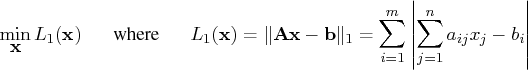
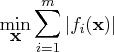
performs linear least absolute value regression by
solving the ![]() norm minimization problem
norm minimization problem
- CALL LAV( rc, xr,
 ,
,  , <x0<,
opt>);
, <x0<,
opt>);
The LAV subroutine returns the following values:
- rc
- is a scalar return code indicating the
reason for optimization termination.
rc Termination 0 Successful 1 Successful, but approximate covariance matrix and standard errors cannot be computed -1 or -3 Unsuccessful: error in the input arguments -2 Unsuccessful: matrix  is rank deficient (
 )
)-4 Unsuccessful: maximum iteration limit exceeded -5 Unsuccessful: no solution found for ill-conditioned problem - xr
- specifies a vector or matrix with
 columns.
If the optimization process is not successfully completed,
xr is a row vector with missing values.
If termination is successful and the opt[3] option is not
set, xr is the vector with the optimal estimate,
columns.
If the optimization process is not successfully completed,
xr is a row vector with missing values.
If termination is successful and the opt[3] option is not
set, xr is the vector with the optimal estimate,  .
If termination is successful and the opt[3] option is
specified, xr is an
.
If termination is successful and the opt[3] option is
specified, xr is an  matrix that contains
the optimal estimate, , in the first row, the asymptotic
standard errors in the second row, and the
matrix that contains
the optimal estimate, , in the first row, the asymptotic
standard errors in the second row, and the  covariance matrix of parameter estimates in the remaining rows.
The inputs to the LAV subroutine are as follows:
- specifies an
 matrix with
 and full column rank,
  .
If you want to include an intercept in the model,
you must include a column of ones in the matrix .
.
If you want to include an intercept in the model,
you must include a column of ones in the matrix . 
- specifies the
 vector
  .
. 
- specifies an optional
 vector that
specifies the starting point of the optimization.
vector that
specifies the starting point of the optimization.
- opt
- is an optional vector used to specify options.
opt[1] specifies the maximum number maxi of outer iterations (this corresponds to the number of changes of the Huber parameter ).
The default is
).
The default is 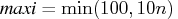 .
(The number of inner iterations is
restricted by an internal threshold.
If the number of inner iterations exceeds this threshold, a new
outer iteration is started with an increased value of .)
.
(The number of inner iterations is
restricted by an internal threshold.
If the number of inner iterations exceeds this threshold, a new
outer iteration is started with an increased value of .)
opt[2] specifies the amount of printed output. Higher values request additional output and include the output of lower values.opt[2] Termination 0 no output is printed 1 error and warning messages are printed 2 the iteration history is printed (this is the default) 3 the least squares ( norm) estimates are printed
if no starting point is specified; the
norm) estimates are printed
if no starting point is specified; the  norm estimates
are printed; if opt[3] is set, the estimates are
printed together with the asymptotic standard errors
norm estimates
are printed; if opt[3] is set, the estimates are
printed together with the asymptotic standard errors4 the approximate covariance matrix of
parameter estimates is printed if opt[3] is set5 the residual and predicted values for all  rows (equations) of are printed
opt[3] specifies which estimate of the variance of the median of nonzero residuals is to be used as a factor for the approximate covariance matrix of parameter estimates and for the approximate standard errors (ASE). If opt![[3]=0](images/langref_langrefeq640.gif) , the McKean-Schrader (1987) estimate
is used, and if opt
, the McKean-Schrader (1987) estimate
is used, and if opt![[3]\gt](images/langref_langrefeq641.gif) , the Cox-Hinkley
(1974) estimate, with
, the Cox-Hinkley
(1974) estimate, with  opt[3], is used.
The default is opt
opt[3], is used.
The default is opt![[3]=-1](images/langref_langrefeq643.gif) or opt
or opt![[3]=.](images/langref_langrefeq644.gif) ,
which means that the covariance matrix is not computed.
,
which means that the covariance matrix is not computed.
opt[4] specifies whether a computationally expensive test for necessary and sufficient optimality of the solution is executed.
The default is opt
is executed.
The default is opt![[4]=0](images/langref_langrefeq645.gif) or opt
or opt![[4]=.](images/langref_langrefeq646.gif) ,
which means that the convergence test is not performed.
,
which means that the convergence test is not performed.
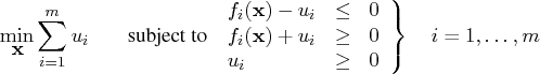
Missing values are not permitted in the
The Least Absolute Values (LAV) subroutine is designed for solving the unconstrained linear
An algorithm by Madsen and Nielsen (1993) is used, which can be faster for large values of
The
- For small values of , you can implement the Nelder-Mead
simplex algorithm with the NLPNMS subroutine to solve
the minimization problem in its original specification.
The Nelder-Mead simplex algorithm does not assume a
smooth objective function, does not take advantage
of any derivatives, and therefore does not require
continuous differentiability of the objective function.
See the section "NLPNMS Call" for details.
- Gonin and Money (1989) describe how an original
 norm estimation problem can be modified to an equivalent
optimization problem with nonlinear constraints which
has a simple differentiable objective function.
You can invoke the NLPQN subroutine, which implements
a quasi-Newton algorithm, to solve the nonlinearly
constrained norm optimization problem.
See the section "NLPQN Call" for details about the NLPQN subroutine.
norm estimation problem can be modified to an equivalent
optimization problem with nonlinear constraints which
has a simple differentiable objective function.
You can invoke the NLPQN subroutine, which implements
a quasi-Newton algorithm, to solve the nonlinearly
constrained norm optimization problem.
See the section "NLPQN Call" for details about the NLPQN subroutine.
Both approaches are successful only for a small number of parameters and good initial estimates. If you cannot supply good initial estimates, the optimal results of the corresponding nonlinear least squares (
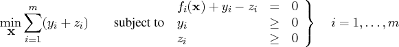
Gonin and Money (1989, pp. 44 - 45) show that the nonlinear
-
 nonlinear
inequality constraints in
nonlinear
inequality constraints in  variables
  and
and  .
. -
nonlinear equality constraints in
 variables
  ,
,  , and .
In addition to computing an optimal solution
The following example is the same one used for illustrating the LAV procedure by Lee and Gentle (1986).
![{a}= [ 1 & 0 \ 1 & 1 \ 1 & -1 \ 1 & -1 \ 1 & 2 \ 1 & 2 ] \hspace*{0.25in} {b}= [ 1 \ 2 \ 1 \ -1 \ 2 \ 4 ]](images/langref_langrefeq666.gif)
    a = { 0,  1, -1, -1,  2,  2 };
    m = nrow(a);
    a = j(m,1,1.) || a;
    b = { 1,  2,  1, -1,  2,  4 };

    opt= { . 5  0 1 };
    call lav(rc,xr,a,b,,opt);
The first part of the printed output refers to the
least squares solution, which is used as the starting point.
The estimates of the largest and smallest nonzero eigenvalues
of The second part of the printed output shows the iteration history.
The third part of the printed output shows the ![]() norm
solution (first row) together with asymptotic standard
errors (second row) and the asymptotic covariance matrix
of parameter estimates (the ASEs are the square roots
of the diagonal elements of this covariance matrix).
norm
solution (first row) together with asymptotic standard
errors (second row) and the asymptotic covariance matrix
of parameter estimates (the ASEs are the square roots
of the diagonal elements of this covariance matrix).
The last part of the printed output shows the predicted values and residuals, as in Lee and Gentle (1986).
Copyright © 2009 by SAS Institute Inc., Cary, NC, USA. All rights reserved.