Language Reference: KALDFF Call :: SAS/IML(R) 9.2 User's Guide

Language Reference

KALDFF Call

computes the one-step forecast of state vectors in an SSM by using the diffuse Kalman filter. The call estimates the conditional expectation of ${z}_t$ , and also estimates the initial random vector, $\delta$ , and its covariance matrix.

CALL KALDFF( pred, vpred, initial, s2, data, lead, int, coef, var,

intd, coefd <, n0, at, mt, qt>);

The inputs to the KALDFF subroutine are as follows:

data: is a matrix containing data $({y}_1, ... , {y}_t)^'$ .
lead: is the number of steps to forecast after the end of the data set.
int: is an $(n_y + n_z) x n_\beta$ matrix for a time-invariant fixed matrix, or a $(t+{lead})(n_y + n_z) x n_\beta$ matrix containing fixed matrices for the time-variant model in the transition equation and the measurement equation - that is, $({w}^'_t, {x}^'_t)^'$ .
coef: is an matrix for a time-invariant coefficient, or a $(t+{lead})(n_y + n_z) x n_z$ matrix containing coefficients at each time in the transition equation and the measurement equation - that is, $({f}^'_t, {h}^'_t)^'$ .
var: is an matrix for a time-invariant variance matrix for the error in the transition equation and the error in the measurement equation, or a $(t+{lead})(n_y + n_z) x (n_y + n_z)$ matrix containing covariance matrices for the error in the transition equation and the error in the measurement equation - that is, $(\eta^'_t, \epsilon^'_t)^'$ .
intd: is an $(n_z + n_\beta) x 1$ vector containing the intercept term in the equation for the initial state vector ${z}_0$ and the mean effect $\beta$ - that is, $({a}^', {b}^')^'$ .
coefd: is an $(n_z + n_\beta) x n_\delta$ matrix containing coefficients for the initial state $\delta$ in the equation for the initial state vector ${z}_0$ and the mean effect $\beta$ - that is, $({a}^', {b}^')^'$ .
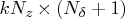
: is an optional scalar including an initial denominator. If $n0\gt$ , the denominator for $\hat{\sigma}^2_t$ is plus the number of elements of $({y}_1, ... , {y}_t)^'$ . If $n0 \leq 0$ or is not specified, the denominator for $\hat{\sigma}^2_t$ is . With $n0 \geq 0$ , the initial values, ${a}_1, {m}_1$ , and ${q}_1$ , are assumed to be known and, hence, , , and are used for input containing the initial values. If the value of is negative or is not specified, the initial values for , , and are computed. The value of is updated as $\max(n0,0) + n_t$ after the KALDFF call.
: is an optional $kn_z x (n_\delta + 1)$ matrix. If $n0 \geq 0$ , contains $({a}^'_1, ... , {a}^'_k)^'$ . However, only the first matrix ${a}_1$ is used as input. When you specify the KALDFF call, returns $({a}^'_{t-k+{lead}+1}, ... , {a}^'_{t+{lead}})^'$ . If is negative or the matrix ${a}_1$ contains missing values, ${a}_1$ is automatically computed.
: is an optional matrix. If $n0 \geq 0$ , contains $({m}_1, ... , {m}_k)^'$ . However, only the first matrix ${m}_1$ is used as input. If is negative or the matrix ${m}_1$ contains missing values, is used for output, and it contains $({m}_{t-k+{lead}+1}, ... , {m}_{t+{lead}})^'$ . Note that the matrix ${m}_1$ can be used as an input matrix if either of the off-diagonal elements is not missing. The missing element ${m}_1(i,j)$ is replaced by the nonmissing element ${m}_1(j,i)$ .
: is an optional $k(n_\delta + 1) x (n_\delta + 1)$ matrix. If $n0 \geq 0$ , contains $({q}_1, ... , {q}_k)^'$ . However, only the first matrix ${q}_1$ is used as input. If is negative or the matrix ${q}_1$ contains missing values, is used for output and contains $({q}_{t-k+{lead}+1}, ... , {q}_{t+{lead}})^'$ . The matrix ${q}_1$ can also be used as an input matrix if either of the off-diagonal elements is not missing since the missing element ${q}_1(i,j)$ is replaced by the nonmissing element ${q}_1(j,i)$ .

The KALDFF call returns the following values:

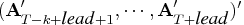
pred: is a $(t+{lead}) x n_z$ matrix containing estimated predicted state vectors $(\hat{{z}}_{1|}, ... , \hat{{z}}_{t+1| t}, \hat{{z}}_{t+2| t}, ... , \hat{{z}}_{t+{lead}| t})^'$ .
vpred: is a $(t+{lead})n_z x n_z$ matrix containing estimated mean square errors of predicted state vectors $({p}_{1|}, ... , {p}_{t+1| t}, {p}_{t+2| t}, ... , {p}_{t+{lead}| t})^'$ .
initial: is an matrix containing an estimate and its variance for initial state $\delta$ , that is, $(\hat{\delta}_t, \hat{\sigma}_{\delta, t})$ .
: is a scalar containing the estimated variance $\hat{\sigma}^2_t$ .

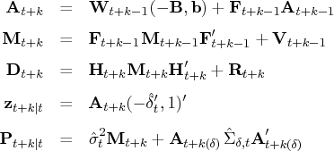
The KALDFF call computes the one-step forecast of state vectors in an SSM by using the diffuse Kalman filter. The SSM for the diffuse Kalman filter is written

${y}_t & = & {x}_t \beta + {h}_t {z}_t + \epsilon_t \ {z}_{t+1} & = & {w}_t \be... ..._t {z}_t + \eta_t \ {z}_0 & = & {a}+ {a}\delta \ \beta & = & {b}+ {b}\delta$

where ${z}_t$ is an

state vector, ${y}_t$ is an

observed vector, and

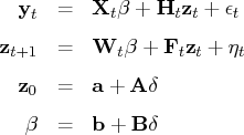
$[ \eta_t \ \epsilon_t ] & \sim & n (0, \sigma^2 [ {v}_t & {g}_t \ {g}^'_t & {{r}}_t ] ) \ \delta & \sim & n(\mu, \sigma^2\sigma)$

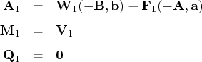
It is assumed that the noise vector $(\eta^'_t, \epsilon^'_t)^'$ is independent and $\delta$ is independent of the vector $(\eta^'_t, \epsilon^'_t)^'$ . The matrices, ${w}_t$ , ${f}_t$ , ${x}_t$ , ${h}_t$ ,

, ${v}_t$ , ${g}_t$ , and ${{r}}_t$ , are assumed to be known. The KALDFF call estimates the conditional expectation of the state vector ${z}_t$ given the observations. The KALDFF subroutine also produces the estimates of the initial random vector $\delta$ and its covariance matrix. For

-step forecasting where $k\gt$ , the estimated conditional expectation at time

is computed with observations given up to time

. The estimated

-step forecast and its estimated MSE are denoted ${z}_{t+k| t}$ and ${p}_{t+k| t}$ (for $k\gt$ ). ${a}_{t+k(\delta)}$ and ${e}_{t(\delta)}$ are last-column-deleted submatrices of ${a}_{t+k}$ and ${e}_t$ , respectively. The algorithm for one-step prediction is given as follows:

${e}_t & = & ({x}_t {b}, {y}_t - {x}_t {b}) - {h}_t {a}_t \ {d}_t & = & {h}_... ...{m}_{t+1} + {a}_{t+1(\delta)} \hat{\sigma}_{\delta,t} {a}^'_{t+1(\delta)}$

where

is the number of elements of $({y}_1, ... , {y}_t)^'$ plus $\max(n0,0)$ . Unless initial values are given and $n0 \geq 0$ , initial values are set as follows:

${a}_1 & = & {w}_1(-{b},{b}) + {f}_1(-{a},{a}) \ {m}_1 & = & {v}_1 \ {q}_1 & = & 0$

For

-step forecasting where $k\gt 1$ ,

${a}_{t+k} & = & {w}_{t+k-1}(-{b},{b}) + {f}_{t+k-1} {a}_{t+k-1} \ {m}_{t+k} ... ...t {m}_{t+k} + {a}_{t+k(\delta)} \hat{\sigma}_{\delta,t} {a}^'_{t+k(\delta)}$

Note that if there is a missing observation, the KALDFF call computes the one-step forecast for the observation following the missing observation as the two-step forecast from the previous observation.

An example that uses the KALDFF call is in the documentation for the KALDFS call.

Top of Page