Biplots
A biplot is a display that attempts to represent both the observations and variables of multivariate data in the same plot. SAS/IML Studio provides biplots as part of the Principal Component analysis.
The computation of biplots in SAS/IML Studio follows the presentation given in Friendly (1991) and Jackson (1991). Detailed discussions of how to compute and interpret biplots are available in Gabriel (1971) and Gower and Hand (1996).
The computation of a biplot begins with the data matrix. If you choose to compute principal components from the covariance matrix (on the Method tab; see Figure 26.3), then the data matrix is centered by subtracting the mean of each column. Otherwise, it is standardized so that each variable has zero mean and unit standard deviation.
In either case, let  denote the resulting
  matrix. The singular value decomposition (SVD) of is the factorization
 |
 |
 |
|||
 |
|
 |
|||
|
|
 |
where  is the diagonal matrix of singular values. If you replace
  and
and  with their first two columns, then an approximate relationship exists:
  . This is a rank-two approximation of . In fact, it is the closest rank-two approximation to in a least squares sense (Golub and Van Loan; 1989).
In a biplot, the rows of the  matrix are plotted as points, which correspond to observations. The rows of the
  matrix are plotted as vectors, which correspond to variables.
The choice of  determines the scaling of the observations and vectors in the biplot. In general, it is impossible to accurately represent the variables and observations in only two dimensions, but you can choose values of that preserve certain properties of the high-dimensional data. Common choices are
  , and
, and  . SAS/IML Studio implements four different versions of the biplot:
- GH

-
This factorization uses
 . This biplot attempts to preserve relationships between variables. This biplot has two useful properties:
 The length of a vector (a row of
) is proportional to the variance of the corresponding variable. The Euclidean distance between the
 th and
  th rows of is proportional to the Mahalanobis distance between the th and th observations in the data set.
- JK
-
This factorization uses
 . This biplot attempts to preserve the distance between observations. This biplot has two useful properties:
 The positions of the points in the biplot are identical to the score plot of first two principal components.
The Euclidean distance between the
th and th rows of G is equal to the Euclidean distance between the th and th observations in the data set.
- SYM
This factorization uses
 . This biplot treats observations and variables symmetrically. This biplot attempts to preserve the values of observations.
 - COV
-
This factorization uses
, but also multiplies by  and divides by the same quantity. This biplot has two useful properties:
The axes at the bottom and left of the biplot are the coordinate axes for the observations. The axes at the top and right of the biplot are the coordinate axes for the vectors.
If the data matrix is not well approximated by a rank-two matrix, then the visual information in the biplot is not a good approximation to the data. In this case, you should not try to interpret the biplot. However, if is close to a rank-two matrix, then you can interpret a biplot in the following ways:
The cosine of the angle between a vector and an axis indicates the importance of the contribution of the corresponding variable to the axis dimension.
The cosine of the angle between vectors indicates correlation between variables. Highly correlated variables point in the same direction; uncorrelated variables are at right angles to each other.
Points that are close to each other in the biplot represent observations with similar values.
You can approximate the coordinates of an observation by projecting the point onto the variable vectors within the biplot.
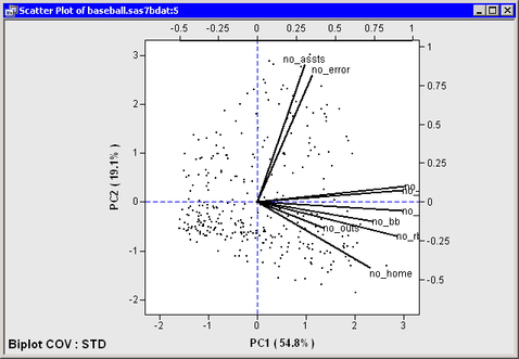
For example, in Figure 26.11 the two principal components account for approximately 74% of the variance in the data. This means that the biplot is a fair (but not good) approximation to the data. The footnote in the plot indicates that the biplot is based on the COV factorization and that the data matrix was standardized (STD).
The variables are grouped: the hitting variables point primarily in the direction of the horizontal axis; no_assts and no_error point primarily in the direction of the vertical axis. The no_outs vector is much shorter than the other vectors, which often indicates that the vector does not lie near the span of the two biplot dimensions.
The hitting variables are strongly correlated with each other. The variables no_assts and no_error are correlated with each other, but they are not correlated with the hitting variables or with no_outs.
Because the biplot is only a moderately good approximation to the data, the following statements are approximately true:
The first and fourth quadrants contain players who tend to be strong hitters. The other quadrants contain weak hitters.
The first and second quadrants contain players who tend to have many assists and errors. The other quadrants contain players with few assists and errors.