Display Attributes
Overview
The display attributes
for the lines, colors, marker symbols, and text used in a graph are
derived from the ODS style that is in effect when the graph is produced.
These display attributes might also be influenced by grouped data.
To override default display attributes, all GTL plot statements provide
options that manage the graph’s visual appearance. For example,
a BOXPLOT statement provides an OUTLIERATTRS= option that manages
the visual appearance of outliers.
-
Change the ODS style that is in effect for the graph. ODS Styles provides an overview of the use of styles in a graph. SAS Graph Template Language: User's Guide discusses the use of styles in more detail.
Display Attributes for Non-Grouped Data
Display Attributes documents the
attribute settings that can be specified for the lines, data markers,
text, or area fills in a plot. The defaults for these attributes are
defined on style elements, but you can use attribute options on the
plot statement to change the defaults.
For example, the LINEPARM statement provides a LINEATTRS=
option that specifies the color, line pattern, or line thickness of
the plot line. For non-grouped data, if you do not set a line pattern
in your template, then the default line pattern for the plot is obtained
from the GraphDataDefault:LineStyle style reference.
To change the default
line pattern, a PATTERN= suboption on LINEATTRS= is available. "Common Line Patterns" shows the most common line patterns available for the PATTERN=
suboption.
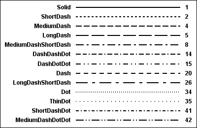
Available Line Patterns provides the complete list of line patterns that can be
used with the GTL.
In the following template
definition, the LINEPARM statement’s LINEATTRS= option overrides
the default line pattern by specifying PATTERN=DASH:
proc template;
  define statgraph patternchange;
    begingraph;
      layout overlay;
        scatterplot y=height x=weight;
        lineparm yintercept=intercept  slope=slope /
          lineattrs=(pattern=dash);
      endlayout;
    endgraph;
  end;
Other display options can be managed the same way. For
example, the SCATTERPLOT statement provides a MARKERATTRS= option
that specifies the color, size, symbol, and weight of the plot data
markers. For non-grouped data, if you do not set a marker symbol in
your template, then the default marker symbol is obtained from the
GraphDataDefault:MarkerSymbol style reference.
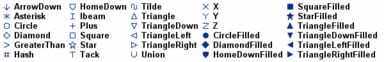
To change the default
marker symbol, a SYMBOL= suboption on MARKERATTRS= is available. "Marker Symbols" shows the marker symbols available for the SYMBOL= suboption.
Display Attributes for Grouped Data
Display Attributes documents the attribute settings that you can specify for
the lines, data markers, text, or area fills in a plot. For grouped
data (that is, when you use the GROUP= option in a plot statement),
each distinct group value can be represented in the graph by a different
combination of line pattern, fill pattern, color, and marker symbol
(depending on the graph type). The defaults for these features are
set by the LineStyle, Color, ContrastColor, FillPattern, and MarkerSymbol
attributes of the GraphData1–GraphDataN style elements.
Note: The MarkerSize and LineThickness
style attributes are not honored in the case of grouped data.
"Common Line Patterns" shows the common line patterns available, and "Marker Symbols" shows the marker symbols available.
For grouped plots, the
style in effect and the plot settings determine which line patterns,
area fills, and plot symbols are used. If different line patterns,
colors, or marker symbols are used to represent group values, then
the style determines the sequences of the line patterns, colors, or
marker symbols that are used for the group values. (As discussed in Cycling through Group Attributes in Overlaid Plots, other plot
settings might also influence the sequence.) If the number of group
values exceeds the number of style elements, the following occurs
for the subsequent group values:
You can use attribute
options on the plot statement to change the default display attributes
used for group data. For example, in the following template definition,
the LINEPARM statement’s LINEATTRS= option specifies PATTERN=DASH.
This explicit setting overrides the default line pattern for the plot
lines and uses dashed lines for all of the plots, leaving color to
distinguish among group values.
proc template;
  define statgraph dashedline;
    begingraph;
      layout overlay;
        scatterplot y=height x=weight / group=gender;
        lineparm yintercept=intercept  slope=slope / group=gender
          lineattrs=(pattern=dash);
      endlayout;
    endgraph;
  end;
Rather than setting
the same line pattern on all group values, you can change the default
sequence of line patterns that is used for grouped values. To do so,
set the LineStyle attribute in some of the style elements GraphData1
through GraphDataN.
In the following example, a style
is defined to change the default line pattern for the first two lines
in the pattern sequence. In this example, the style is derived from
the DEFAULT style, which is available for the HTML destination. Values
are set for the LineStyle attributes in the GraphData1 and GraphData2
style elements. The first default line in the sequence has long dashes
(style value 6) and the second line has short dashes (style value
4). The LineStyle settings for the remaining GraphData elements are
not set, so are derived from the parent style (DEFAULT). This new
line sequence is used as the default line sequence for any plot that
uses the MyDefault style. To apply the style to a graph, the STYLE=
option is used in the ODS HTML statement to specify the style name.
/* Sort the SASHELP.CLASS data by sex and age. */
proc sort data=sashelp.class(keep=height weight sex age)
     out=class;
  by sex age;
run;

/* Generate slope and intercept data for plot reference lines. */
proc robustreg data=class method=m
      outest=stats(rename=(weight=slope));
   by sex;
   model height=weight;
run;

data class;
   merge class stats(keep=intercept slope sex);
run;

proc template;
   /* Create custom style STYLES.MYDEFAULT from the STYLES.DEFAULT style. */
   define style Styles.MyDefault;
      parent=Styles.Default;
      style GraphData1 from GraphData1 /
         LineStyle=6;
      style GraphData2 from GraphData2 /
         LineStyle=4;
   end;

   /* Create the plot template. */
   define statgraph testPattern;
      begingraph;
         layout overlay;
            scatterplot y=height x=weight / group=sex;
            lineparm x=0 y=intercept slope=slope / group=sex name="lines";
            discretelegend "lines";
         endlayout;
      endgraph;
    end;
run;

/* Generate the plot. */
ods _all_ close;
ods html style=MyDefault; /* Apply style MyDefault to the graph. */

proc sgrender data=class template=testPattern;
run;
Similarly, for grouped
data, you can set the MarkerSymbol attribute in each of the style
elements GraphData1 through GraphDataN. In the following example,
a style is defined to change the default sequence that is used for
the first three marker symbols in grouped plots. Values are set for
the MarkerSymbol attributes in the GraphData1 through GraphData3 style
elements. This new sequence is used as the default marker symbol sequence
for any plot that uses the MyDefault style.
proc template;
   /* Create custom style STYLES.MYDEFAULT from the STYLES.DEFAULT style. */
   define style Styles.MyDefault;
      parent=Styles.Default;
      style GraphData1 from GraphData1 /
         MarkerSymbol="DIAMOND";
      style GraphData2 from GraphData2 /
         MarkerSymbol="CROSS";
      style GraphData3 from GraphData3 /
         MarkerSymbol="CIRCLE";
   end;

   /* Create the plot template. */
   define statgraph testSymbols;
      begingraph;
         layout Overlay;
            scatterPlot y=height x=weight / group=age name="symbols";
            discretelegend "symbols" / title="Age";
         endlayout;
      endgraph;
   end;
run;

/* Generate the plot. */
ods html close;
ods html style=MyDefault; /* Apply style MyDefault to the graph. */

proc sgrender data=class template=testSymbols;
run;
Cycling through Group Attributes in Overlaid Plots
Overlay-type layouts
provide the CYCLEATTRS= options that specifies whether the default
visual attributes of lines, marker symbols, and area fills in nested
plot statements automatically change from plot to plot. When CYCLEATTRS=TRUE,
all applicable plot statements (SCATTERPLOT, SERIESPLOT, and others)
are sequentially assigned the next unused GraphDataN style element.
(The sequence is overridden for plot statements that have an explicit
setting, either through a style element assignment or option settings.)
No plot retains its default (implicit) style element.
In the following example,
assuming ungrouped data, the series plots are assigned line properties
based on the GraphData1, GraphData2, and GraphData3 style elements.
The reference line uses GraphReference, not GraphData4.
layout overlay / cycleattrs=true;
  seriesplot x=date y=var1;
  seriesplot x=date y=var2;
  seriesplot x=date y=var3;
  referenceline x=cutoff / lineattrs=GraphReference;
endlayout;
If one of the plots
in this example uses grouped data, the grouped plots also participate
in the default cycles. For example, if the second plot has three groups,
it generates three plots, which are assigned line properties based
on the GraphData2, GraphData3, and GraphData4 style elements.
If the plot statement
that uses grouped data also uses the INDEX= option to manage the group
values (see Remapping Groups for Grouped Data), the INDEX=
option overrides the default behavior. In that case, the grouped plots
do not participate in the default cycling.
Remapping Groups for Grouped Data
Indexing can be
used to collapse the number of groups that are represented in a graph.
For example, if 10 groups are in the data, indexes 1 and 2 can be
assigned to the first two groups, and index 3 can be assigned to all
other groups. The third through tenth data groups are treated as a
single group in the graph.
Indexing can control
the order in which colors, area fills, marker symbols, and line styles
are mapped to group values in a graph. This ordering method is needed
only for coordinating the data display of multiple graphs when the
default mapping would cause group values to be mismatched between
graphs.
For example, consider
two studies of three drugs, A, B, and C. If Study 1 uses all three
drugs, then the first combination of color and marker symbol is mapped
to Drug A. The second combination of color and marker symbol is mapped
to Drug B, and the third is mapped to Drug C. If Study 2 omits Drug
A, then the first combination of color and marker symbol is mapped
to Drug B, and the second is mapped to Drug C. If the two graphs are
viewed together, then this default mapping causes the group values
to be mismatched. The visual attributes that represent Drug A in the
first graph represent Drug B in the second graph. Those that represent
Drug B in the first graph represent Drug C in the second group.
Interactions between Options
When you use GTL statement
options to manage the graph display, interactions between options
might cause some option settings to be ignored. For example, an ENTRYTITLE
statement provides BORDER= and BORDERATTRS= options for managing a
border line around the graph title. Border attributes that are set
on the BORDERATTRS= option have no effect on the graph title unless
the title border line is displayed by setting BORDER=TRUE.
Similarly, if a BOXPLOT
statement’s DISPLAY= option suppresses the display of outliers
in a box plot, then using the OUTLIERATTRS= option to set outlier
attributes has no effect. The OUTLIERATTRS= settings only take effect
if DISPLAY= enables the display of outliers.