Using Predictor Variables

You have now defined three interventions to model the changes in trend and level. The excursion near the end of the series remains to be dealt with.

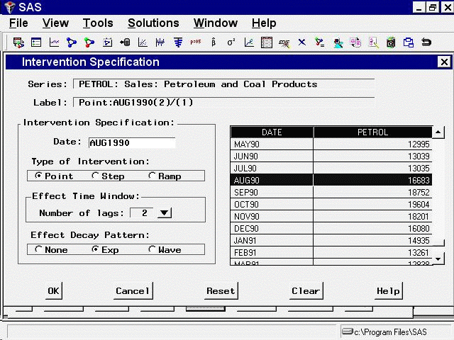
Select Add from the Interventions for Series window. Scroll through the data values and select the date on which the excursion began, August 1990. Leave the intervention type as Point.

The pattern of the series from August 1990 through January 1991 is more complex than a simple shift in level or trend. For this pattern, you need a complex intervention model for an event that causes a sharp rise followed by a rapid return to the previous trend line. To specify this model, use the Effect Time Window and Effect Decay Rate options.

The Effect Time Window option controls the number of lags of the intervention’s indicator variable used to model the effect of the intervention on the dependent series. For a simple intervention, the number of lags is zero, which means that the effect of the intervention is modeled by fitting a single regression coefficient to the intervention’s indicator variable.

When you set the number of lags greater than zero, regression coefficients are fit to lags of the indicator variable. This allows you to model interventions whose effects take place gradually, or to model rebound effects. For example, severe weather might reduce production during one period but cause an increase in production in the following period as producers struggle to catch up. You could model this by using a point intervention with an effect time window of 1 lag. This would fit two coefficients for the intervention, one for the immediate effect and one for the delayed effect.

The Effect Decay Pattern option controls how the effect of the intervention dissipates over time. None specifies that there is no gradual decay: for point interventions, the effect ends immediately; for step and ramp interventions, the effect continues indefinitely. Exp specifies that the effect declines at an exponential rate. Wave specifies that the effect declines like an exponentially damped sine wave (or as the sum of two exponentials, depending on the fit to the data).

If you are familiar with time series analysis, these options might be clearer if you note that together the Effect Time Window and Effect Decay Pattern options define the numerator and denominator orders of a transfer function or dynamic regression model for the indicator variable of the intervention. See the section Dynamic Regressor for more information.

For this example, select 2 lags as the value of the Event Time Window option, and select Exp as the Effect Decay Pattern option. The window should now appear as shown in Figure 58.20.

Select the OK button to add the intervention to the list.