Using Predictor Variables

Selecting Dynamic Regressor from the Add Predictors menu (shown in Figure 58.1) allows you to specify a complex time series model of the way that a predictor variable influences the series that you are forecasting.

When you specify a predictor variable as a simple regressor, only the current period value of the predictor effects the forecast for the period. By specifying the predictor with the Dynamic Regression option, you can use past values of the predictor series, and you can model effects that take place gradually.

Dynamic regression models are an advanced feature that you are unlikely to find useful unless you have studied the theory of statistical time series analysis. You might want to skip this section if you are not trained in time series modeling.

The term dynamic regression was introduced by Pankratz (1991) and refers to what Box and Jenkins (1976) named transfer function models. In dynamic regression, you have a time series model, similar to an ARIMA model, that predicts how changes in the predictor series affect the dependent series over time.

The dynamic regression model relates the predictor variable to the expected value of the dependent series in the same way that an ARIMA model relates the fluctuations of the dependent series about its conditional mean to the random error term (which is also called the innovation series). For more information about dynamic regression or transfer function see Pankratz (1991); Box and Jenkins (1976). See also Chapter 8: The ARIMA Procedure.

From the Develop Models window, select Fit ARIMA Model. From the ARIMA Model Specification window, select Add and then select Linear Trend from the menu (shown in Figure 58.1).

Now select Add and select Dynamic Regressor. This displays the Dynamic Regressors Selection window, as shown in Figure 58.11.

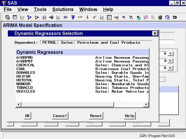
You can select only one predictor series when specifying a dynamic regression model. For this example, select VEHICLES, Sales: Motor Vehicles and Parts. Then select the OK button.

This displays the Dynamic Regression Specification window, as shown in Figure 58.12.

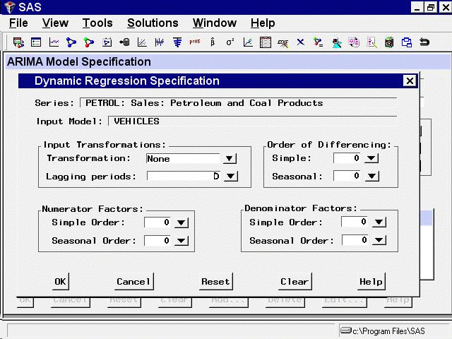
This window consists of four parts. The Input Transformations fields enable you to transform or lag the predictor variable. For example, you might use the lagged logarithm of the variable as the predictor series.

The Order of Differencing fields enable you to specify simple and seasonal differencing of the predictor series. For example, you might use changes in the predictor variable instead of the variable itself as the predictor series.

The Numerator Factors and Denominator Factors fields enable you to specify the orders of simple and seasonal numerator and denominator factors of the transfer function.

Simple regression is a special case of dynamic regression in which the dynamic regression model consists of only a single regression coefficient for the current value of the predictor series. If you select the OK button without specifying any options in the Dynamic Regression Specification window, a simple regressor will be added to the model.

For this example, use the Simple Order combo box for Denominator Factors and set its value to 1. The window now appears as shown in Figure 58.13.

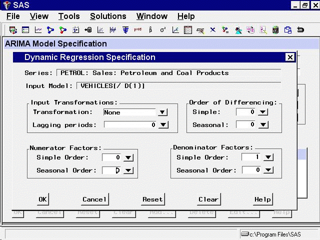
This model is equivalent to regression on an exponentially weighted infinite distributed lag of VEHICLES (in the same way an MA(1) model is equivalent to single exponential smoothing).

Select the OK button to add the dynamic regressor to the model predictors list.

In the ARIMA Model Specification window, the Predictors list should now contain two items, a linear trend and a dynamic regressor for VEHICLES, as shown in Figure 58.14.

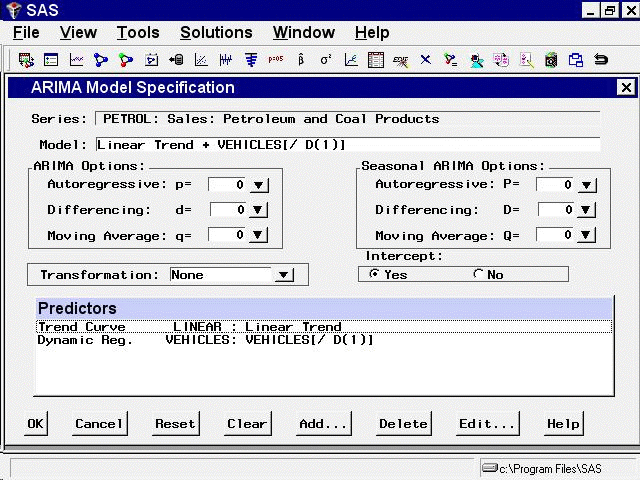
This model is a multiple regression of PETROL on a time trend variable and an infinite distributed lag of VEHICLES. Select the OK button to fit the model.

As with simple regressors, if VEHICLES does not already have a forecasting model, an automatic model selection process is performed to find a forecasting model for VEHICLES before the dynamic regression model for PETROL is fit.