The MDC Procedure

Nested Logit

The nested logit model (McFadden 1978, 1981) allows partial relaxation of the assumption of independence of the stochastic components of utility of alternatives. In some choice situations, the IIA property holds for some pairs of alternatives but not all. In these situations, the nested logit model can be used if the set of alternatives faced by an individual can be partitioned into subsets such that the IIA property holds within subsets but not across subsets.

In the nested logit model, the joint distribution of the errors is generalized extreme value (GEV). This is a generalization of the Type I extreme-value distribution that gives rise to the conditional logit model. Note that all $\epsilon _{ij}$ within each subset are correlated with each other. Refer to McFadden (1978, 1981) for details.

Nested logit models can be described analytically following the notation of McFadden (1981). Assume that there are L levels, with 1 representing the lowest and L representing the highest level of the tree. The index of a node at level h in the tree is a pair 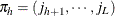$(j_{h}, \pi _{h})$ , where $\pi _{h} = (j_{h+1},\cdots , j_{L})$ is the index of the adjacent node at level $h+1$ . Thus, the primitive alternatives, at level 1 in the tree, are indexed by vectors $(j_{1},\cdots , j_{L})$ , and the alternative nodes at level L are indexed by integers $j_{L}$ . The choice set $C_{\pi _{h}}$ is the set of primitive alternatives (at level 1) that belong to branches below the node $\pi _{h}$ . The notation $C_{\pi _{h}}$ is also used to denote a set of indices $j_{h}$ such that $(j_{h},\pi _{h})$ is a node immediately below $\pi _{h}$ . 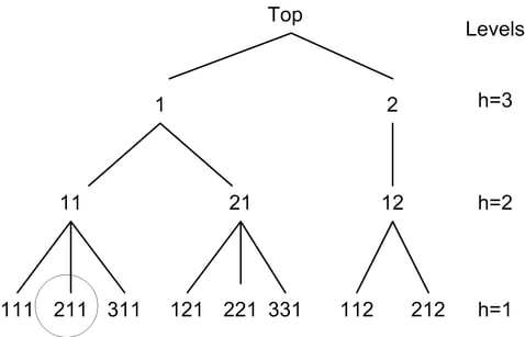Note that $C_{\pi _{0}}$ is a set with a single element, while $C_{\pi _{L}}$ represents a choice set that contains all possible alternatives. As an example, consider the circled node at level 1 in Figure 25.26. Since it stems from node 11, $\pi _{h}=11$ , and since it is the second node stemming from 11, $j_ h=2$ , its index is $\pi _{h-1}=\pi _0=(j_ h, \pi _ h)=211$ . Similarly, 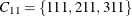$C_{11}=\{ 111, 211, 311\}$ contains all the possible choices below 11.

Although this notation is useful for writing closed-form solutions for probabilities, the MDC procedure allows a more flexible definition of indices. See the section NEST Statement for more details about how to describe decision trees within the MDC procedure.

Figure 25.26: Node Indices for a Three-Level Tree

Let $\mathbf{x}_{i;j_{h}\pi _{h}}^{(h)}$ denote the vector of observed variables for individual i common to the alternatives below node $j_{h}\pi _{h}$ . The probability of choice at level h has a closed-form solution and is written

$P_{i}(j_{h}|\pi _{h}) = \frac{\exp \left[\mathbf{x}_{i;j_{h}\pi _{h}}^{(h)\prime } \bbeta ^{(h)}+\sum _{k\in C_{i;j_{h}\pi _{h}}}I_{k,j_{h}\pi _{h}} \theta _{k,j_{h}\pi _{h}}\right]}{\sum _{j\in C_{i;\pi _{h}}} \exp \left[\mathbf{x}_{i;j\pi _{h}}^{(h)\prime }\bbeta ^{(h)}+\sum _{k\in C_{i;j\pi _{h}}} I_{k,j\pi _{h}}\theta _{k,j\pi _{h}}\right]},h=2,\cdots ,L$

where $I_{\pi _ h}$ is the inclusive value (at level $h+1$ ) of the branch below node $\pi _{h}$ and is defined recursively as follows:

$I_{\pi _{h}} = \ln \left\{ \sum _{j\in C_{i;\pi _{h}}} \exp \left[\mathbf{x}_{i;j\pi _{h}}^{(h)\prime }\bbeta ^{(h)}+ \sum _{k\in C_{i;j\pi _{h}}}I_{k,j\pi _{h}}\theta _{k,j\pi _{h}}\right] \right\}$

$0 \leq \theta _{k,\pi _{1}} \leq \cdots \leq \theta _{k,\pi _{L-1}}$

The inclusive value $I_{\pi _ h}$ denotes the average utility that the individual can expect from the branch below $\pi _ h$ . The dissimilarity parameters or inclusive value parameters ( $\theta _{k,j\pi _{h}}$ ) are the coefficients of the inclusive values and have values between 0 and 1 if nested logit is the correct model specification. When they all take value 1, the nested logit model is equivalent to the conditional logit model.

At decision level 1, there is no inclusive value; that is, $I_{\pi _{0}}=0$ . Therefore, the conditional probability is

$P_{i}(j_{1}|\pi _{1}) = \frac{\exp \left[\mathbf{x}_{i;j_{1}\pi _{1}}^{(1)\prime } \bbeta ^{(1)}\right]}{\sum _{j\in C_{i;\pi _{1}}}\exp \left[\mathbf{x}_{i;j\pi _{1}}^{(1)\prime } \bbeta ^{(1)}\right]}$

The log-likelihood function at level h can then be written

$\mathcal{L}^{(h)} = \sum _{i=1}^{N}\sum _{\pi _{h'}\in C_{i,\pi _{h+1}}} \sum _{j\in C_{i,\pi _{h'}}}y_{i,j\pi _{h'}}\ln P(C_{i,j\pi _{h'}}|C_{i,\pi _{h'}})$

where $y_{i,j\pi _{h'}}$ is an indicator variable that has the value of 1 for the selected choice. The full log-likelihood function of the nested logit model is obtained by adding the conditional log-likelihood functions at each level:

$\mathcal{L} = \sum _{h=1}^{L}\mathcal{L}^{(h)}$

Note that the log-likelihood functions are computed from conditional probabilities when $h<L$ . The nested logit model is estimated using the full information maximum likelihood method.