The FORECAST Procedure
- Overview
-
Getting Started
 Giving Dates to Forecast ValuesComputing Confidence LimitsForm of the OUT= Data SetPlotting ForecastsPlotting ResidualsModel Parameters and Goodness-of-Fit StatisticsControlling the Forecasting MethodIntroduction to Forecasting MethodsTime Trend ModelsTime Series MethodsCombining Time Trend with Autoregressive Models
 -
Syntax
-
Details
-
Examples
- References
OUTEST= Data Set
The FORECAST procedure writes the parameter estimates and goodness-of-fit statistics to an output data set when the OUTEST= option is specified. The OUTEST= data set contains the following variables:
-
the BY variables
-
the first ID variable, which contains the value of the ID variable for the last observation in the input data set used to fit the model
-
_TYPE_, a character variable that identifies the type of each observation
-
the VAR statement variables, which contain statistics and parameter estimates for the input series. The values contained in the VAR statement variables depend on the _TYPE_ variable value for the observation.
The observations contained in the OUTEST= data set are identified by the _TYPE_ variable. The OUTEST= data set might contain observations with the following _TYPE_ values:
- AR1–ARn
-
The observation contains estimates of the autoregressive parameters for the series. Two-digit lag numbers are used if the value of the NLAGS= option is 10 or more; in that case these _TYPE_ values are AR01–ARn. These observations are output for the STEPAR method only.
- CONSTANT
-
The observation contains the estimate of the constant or intercept parameter for the time trend model for the series. For the exponential smoothing and the Winters’ methods, the trend model is centered (that is, t =0) at the last observation used for the fit.
- LINEAR
-
The observation contains the estimate of the linear or slope parameter for the time trend model for the series. This observation is output only if you specify TREND=2 or TREND=3.
- N
-
The observation contains the number of nonmissing observations used to fit the model for the series.
- QUAD
-
The observation contains the estimate of the quadratic parameter for the time trend model for the series. This observation is output only if you specify TREND=3.
- SIGMA
-
The observation contains the estimate of the standard deviation of the error term for the series.
- S1–S3
-
The observations contain exponentially smoothed values at the last observation. _TYPE_=S1 is the final smoothed value of the single exponential smooth. _TYPE_=S2 is the final smoothed value of the double exponential smooth. _TYPE_=S3 is the final smoothed value of the triple exponential smooth. These observations are output for METHOD=EXPO only.
- S_name
-
The observation contains estimates of the seasonal parameters. For example, if SEASONS=MONTH, the OUTEST= data set contains observations with _TYPE_=S_JAN, _TYPE_=S_FEB, _TYPE_=S_MAR, and so forth.
For multiple-period seasons, the names of the first and last interval of the season are concatenated to form the season name. Thus, for SEASONS=MONTH4, the OUTEST= data set contains observations with _TYPE_=S_JANAPR, _TYPE_=S_MAYAUG, and _TYPE_=S_SEPDEC.
When the SEASONS= option specifies numbers, the seasonal factors are labeled _TYPE_=S_i_j. For example, SEASONS=(2 3) produces observations with _TYPE_ values of S_1_1, S_1_2, S_2_1, S_2_2, and S_2_3. The observation with _TYPE_=S_i_j contains the seasonal parameters for the jth season of the ith seasonal cycle.
These observations are output only for METHOD=WINTERS or METHOD=ADDWINTERS.
- WEIGHT
-
The observation contains the smoothing weight used for exponential smoothing. This is the value of the WEIGHT= option. This observation is output for METHOD=EXPO only.
- WEIGHT1 | WEIGHT2 | WEIGHT3
-
The observations contain the weights used for smoothing the WINTERS or ADDWINTERS method parameters (specified by the WEIGHT= option). _TYPE_=WEIGHT1 is the weight used to smooth the CONSTANT parameter. _TYPE_=WEIGHT2 is the weight used to smooth the LINEAR and QUAD parameters. _TYPE_=WEIGHT3 is the weight used to smooth the seasonal parameters. These observations are output only for the WINTERS and ADDWINTERS methods.
- NRESID
-
The observation contains the number of nonmissing residuals, n, used to compute the goodness-of-fit statistics. The residuals are obtained by subtracting the one-step-ahead predicted values from the observed values.
- SST
-
The observation contains the total sum of squares for the series, corrected for the mean.
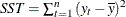 , where
  is the series mean.
- SSE
-
The observation contains the sum of the squared residuals, uncorrected for the mean.
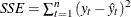 , where
  is the one-step predicted value for the series.
- MSE
-
The observation contains the mean squared error, calculated from one-step-ahead forecasts.
 , where k is the number of parameters in the model.
- RMSE
-
The observation contains the root mean squared error.
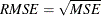 .
.
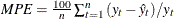
- MAPE
-
The observation contains the mean absolute percent error.
 .
.
- MPE
-
The observation contains the mean percent error.
 .
.
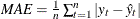
- MAE
-
The observation contains the mean absolute error.
 .
.
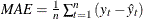
- ME
-
The observation contains the mean error.
 .
.
- MAXE
-
The observation contains the maximum error (the largest residual).
- MINE
-
The observation contains the minimum error (the smallest residual).
- MAXPE
-
The observation contains the maximum percent error.
- MINPE
-
The observation contains the minimum percent error.
- RSQUARE
-
The observation contains the R square statistic,
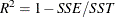 . If the model fits the series badly, the model error sum of squares SSE might be larger than SST and the R square statistic will be negative.
- ADJRSQ
-
The observation contains the adjusted R square statistic.
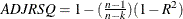 .
.
- ARSQ
-
The observation contains Amemiya’s adjusted R square statistic.
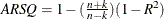 .
.
- RW_RSQ
-
The observation contains the random walk R square statistic (Harvey’s
 statistic that uses the random walk model for comparison).
 ,
,
where
 and
and 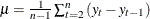 .
.
- AIC
-
The observation contains Akaike’s information criterion.
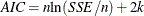 .
.
- SBC
-
The observation contains Schwarz’s Bayesian criterion.
 .
.
- APC
-
The observation contains Amemiya’s prediction criterion.
 .
.
- CORR
-
The observation contains the correlation coefficient between the actual values and the one-step-ahead predicted values.
- THEILU
-
The observation contains Theil’s U statistic that uses original units. See Maddala (1977, pp. 344–345), and Pindyck and Rubinfeld (1981, pp. 364–365) for more information about Theil statistics.
- RTHEILU
-
The observation contains Theil’s U statistic calculated using relative changes.
- THEILUM
-
The observation contains the bias proportion of Theil’s U statistic.
- THEILUS
-
The observation contains the variance proportion of Theil’s U statistic.
- THEILUC
-
The observation contains the covariance proportion of Theil’s U statistic.
- THEILUR
-
The observation contains the regression proportion of Theil’s U statistic.
- THEILUD
-
The observation contains the disturbance proportion of Theil’s U statistic.
- RTHEILUM
-
The observation contains the bias proportion of Theil’s U statistic, calculated by using relative changes.
- RTHEILUS
-
The observation contains the variance proportion of Theil’s U statistic, calculated by using relative changes.
- RTHEILUC
-
The observation contains the covariance proportion of Theil’s U statistic, calculated by using relative changes.
- RTHEILUR
-
The observation contains the regression proportion of Theil’s U statistic, calculated by using relative changes.
- RTHEILUD
-
The observation contains the disturbance proportion of Theil’s U statistic, calculated by using relative changes.