The TIMESERIES Procedure
- Overview
- Getting Started
-
Syntax

-
DetailsAccumulationMissing Value InterpretationTime Series TransformationTime Series DifferencingDescriptive StatisticsSeasonal DecompositionCorrelation AnalysisCross-Correlation AnalysisSpectral Density AnalysisSingular Spectrum AnalysisData Set OutputOUT= Data SetOUTCORR= Data SetOUTCROSSCORR= Data SetOUTDECOMP= Data SetOUTPROCINFO= Data SetOUTSEASON= Data SetOUTSPECTRA= Data SetOUTSSA= Data SetOUTSUM= Data SetOUTTREND= Data Set_STATUS_ Variable ValuesPrinted OutputODS Table NamesODS Graphics Names
-
Examples
- References
Example 33.2 Trend and Seasonal Analysis
This example illustrates using the TIMESERIES procedure for trend and seasonal analysis of time-stamped transactional data.
Suppose that the data set SASHELP.AIR contains two variables: DATE and AIR. The variable DATE contains sorted SAS date values recorded at no particular frequency. The variable AIR contains the transaction values to be analyzed.
The following statements accumulate the transactional data on an average basis to form a quarterly time series and perform trend and seasonal analysis on the transactions.
proc timeseries data=sashelp.air
                out=series
                outtrend=trend
                outseason=season print=seasons;
   id date interval=qtr accumulate=avg;
   var air;
run;
The time series is stored in the data set WORK.SERIES, the trend statistics are stored in the data set WORK.TREND, and the seasonal statistics are stored in the data set WORK.SEASON. Additionally, the seasonal statistics are printed (PRINT=SEASONS) and the results of the seasonal analysis are shown in Output 33.2.1.
Output 33.2.1: Seasonal Statistics Table
| Season Statistics for Variable AIR | ||||||
|---|---|---|---|---|---|---|
| Season Index | N | Minimum | Maximum | Sum | Mean | Standard Deviation |
| 1 | 36 | 112.0000 | 419.0000 | 8963.00 | 248.9722 | 95.65189 |
| 2 | 36 | 121.0000 | 535.0000 | 10207.00 | 283.5278 | 117.61839 |
| 3 | 36 | 136.0000 | 622.0000 | 12058.00 | 334.9444 | 143.97935 |
| 4 | 36 | 104.0000 | 461.0000 | 9135.00 | 253.7500 | 101.34732 |
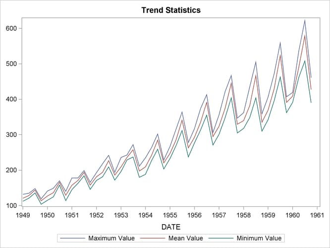
Using the trend statistics stored in the WORK.TREND data set, the following statements plot various trend statistics associated with each time period over time.
title1 "Trend Statistics";
proc sgplot data=trend;
   series x=date y=max  / lineattrs=(pattern=solid);
   series x=date y=mean / lineattrs=(pattern=solid);
   series x=date y=min  / lineattrs=(pattern=solid);
   yaxis display=(nolabel);
   format date year4.;
run;
The results of this trend analysis are shown in Output 33.2.2.
Output 33.2.2: Trend Statistics Plot
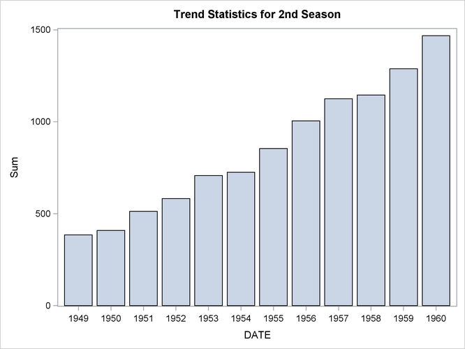
Using the trend statistics stored in the WORK.TREND data set, the following statements chart the sum of the transactions associated with each time period for the second season
over time.
title1 "Trend Statistics for 2nd Season";
proc sgplot data=trend;
   where _season_ = 2;
   vbar date / freq=sum;
   format date year4.;
   yaxis label='Sum';
run;
The results of this trend analysis are shown in Output 33.2.3.
Output 33.2.3: Trend Statistics Bar Chart
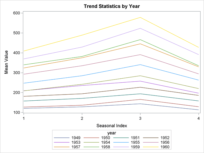
Using the trend statistics stored in the WORK.TREND data set, the following statements plot the mean of the transactions associated with each time period by each year over time.
data trend;
   set trend;
   year = year(date);
run;

title1 "Trend Statistics by Year";
proc sgplot data=trend;
   series x=_season_ y=mean / group=year lineattrs=(pattern=solid);
   xaxis values=(1 to 4 by 1);
run;
The results of this trend analysis are shown in Output 33.2.4.
Output 33.2.4: Trend Statistics
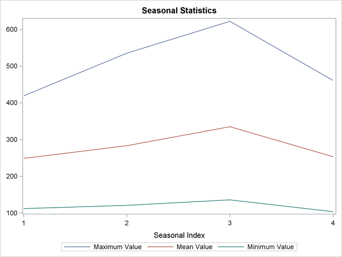
Using the season statistics stored in the WORK.SEASON data set, the following statements plot various season statistics for each season.
title1 "Seasonal Statistics";
proc sgplot data=season;
   series x=_season_ y=max  / lineattrs=(pattern=solid);
   series x=_season_ y=mean / lineattrs=(pattern=solid);
   series x=_season_ y=min  / lineattrs=(pattern=solid);
   yaxis display=(nolabel);
   xaxis values=(1 to 4 by 1);
run;
The results of this seasonal analysis are shown in Output 33.2.5.
Output 33.2.5: Seasonal Statistics Plot