The SEVERITY Procedure
- Overview
-
Getting Started

-
Syntax
-
DetailsPredefined DistributionsCensoring and TruncationParameter Estimation MethodParameter InitializationEstimating Regression EffectsEmpirical Distribution Function Estimation MethodsStatistics of FitDefining a Distribution Model with the FCMP ProcedurePredefined Utility FunctionsCustom Objective FunctionsMultithreaded ComputationInput Data SetsOutput Data SetsDisplayed OutputODS Graphics
-
Examples
- References
An Example with Left-Truncation and Right-Censoring
PROC SEVERITY enables you to specify that the response variable values are left-truncated or right-censored. The following
DATA step expands the data set of the previous example to simulate a scenario that is typically encountered by an automobile
insurance company. The values of the variable Y represent the loss values on claims that are reported to an auto insurance company. The variable THRESHOLD records the deductible on the insurance policy. If the actual value of Y is less than or equal to the deductible, then it is unobservable and does not get recorded. In other words, THRESHOLD specifies the left-truncation of Y. LIMIT records the policy limit. If the value of Y is equal to or greater than the recorded value, then the observation is right-censored.
/*----- Lognormal Model with left-truncation and censoring -----*/
data test_sev2(keep=y threshold limit
        label='A Lognormal Sample With Censoring and Truncation');
   set test_sev1;
   label y='Censored & Truncated Response';
   if _n_ = 1 then call streaminit(45679);

   /* make about 20% of the observations left-truncated */
   if (rand('UNIFORM') < 0.2) then
      threshold = y * (1 - rand('UNIFORM'));
   else
      threshold = .;
   /* make about 15% of the observations right-censored */
   iscens = (rand('UNIFORM') < 0.15);
   if (iscens) then
      limit = y;
   else
      limit = .;
run;
The following statements use the AICC criterion to analyze which of the four predefined distributions (lognormal, Burr, gamma, and Weibull) has the best fit for the data:
proc severity data=test_sev2 crit=aicc
       print=all plots=(cdfperdist pp qq);
   loss y / lt=threshold rc=limit;

   dist logn burr gamma weibull;
run;
The LOSS statement specifies the left-truncation and right-censoring variables. Each candidate distribution needs to be specified by using a separate DIST statement. The PRINT= option in the PROC SEVERITY statement requests that all the displayed output be prepared. The PLOTS= option in the PROC SEVERITY statement requests that the CDF plot, P-P plot, and Q-Q plot be prepared for each candidate distribution in addition to the default plots.
Some of the key results prepared by PROC SEVERITY are shown in Figure 23.6 through Figure 23.13. In addition to the estimates of the range, mean, and standard deviation of Y, the “Descriptive Statistics for Y” table shown in Figure 23.6 also indicates the number of observations that are left-truncated or right-censored. The “Model Selection Table” in Figure 23.6 shows that models with all the candidate distributions have converged and that the Logn (lognormal) model has the best fit
for the data according to the AICC criterion.
Figure 23.6: Summary Results for the Truncated and Censored Data
| Input Data Set | |
|---|---|
| Name | WORK.TEST_SEV2 |
| Label | A Lognormal Sample With Censoring and Truncation |
| Descriptive Statistics for Variable y | |
|---|---|
| Number of Observations | 100 |
| Number of Observations Used for Estimation | 100 |
| Minimum | 2.30264 |
| Maximum | 8.34116 |
| Mean | 4.62007 |
| Standard Deviation | 1.23627 |
| Number of Left Truncated Observations | 23 |
| Number of Right Censored Observations | 14 |
| Model Selection Table | |||
|---|---|---|---|
| Distribution | Converged | Corrected Akaike's Information Criterion |
Selected |
| Logn | Yes | 298.92672 | Yes |
| Burr | Yes | 302.66229 | No |
| Gamma | Yes | 299.45293 | No |
| Weibull | Yes | 309.26779 | No |
PROC SEVERITY also prepares a table that shows all the fit statistics for all the candidate models. It is useful to see which model would be the best fit according to each of the criteria. The “All Fit Statistics Table” prepared for this example is shown in Figure 23.7. It indicates that the lognormal model is chosen by all the criteria.
Figure 23.7: Comparing All Statistics of Fit for the Truncated and Censored Data
| All Fit Statistics Table | ||||||||||||||
|---|---|---|---|---|---|---|---|---|---|---|---|---|---|---|
| Distribution | -2 Log Likelihood |
AIC | AICC | BIC | KS | AD | CvM | |||||||
| Logn | 294.80301 | * | 298.80301 | * | 298.92672 | * | 304.01335 | * | 0.51824 | * | 0.34736 | * | 0.05159 | * |
| Burr | 296.41229 | 302.41229 | 302.66229 | 310.22780 | 0.66984 | 0.36712 | 0.05726 | |||||||
| Gamma | 295.32921 | 299.32921 | 299.45293 | 304.53955 | 0.62511 | 0.42921 | 0.05526 | |||||||
| Weibull | 305.14408 | 309.14408 | 309.26779 | 314.35442 | 0.93307 | 1.40699 | 0.17465 | |||||||
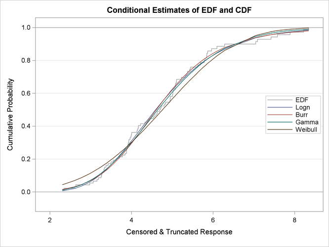
The plot that compares EDF and CDF estimates is shown in Figure 23.8. When left-truncation is specified, both the EDF and CDF estimates are conditional on the response variable being greater than the smallest left-truncation threshold in the sample.
Figure 23.8: EDF and CDF Estimates for the Truncated and Censored Data
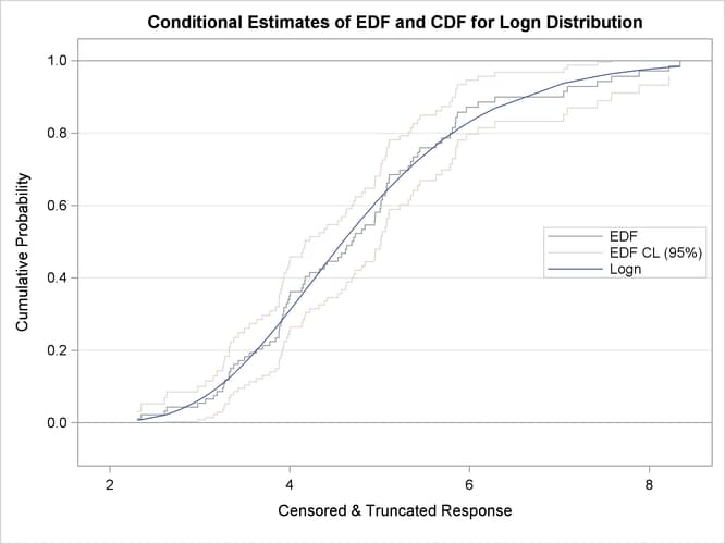
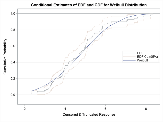
When you specify the PLOTS=CDFPERDIST option, PROC SEVERITY prepares a plot that compares the nonparametric EDF estimates with the parametric CDF estimates for each distribution. These plots for lognormal and Weibull distributions are shown in Figure 23.9. These plots also contain the lower and upper confidence limits of EDF for the specified confidence level. Because no confidence level was specified in the EDFALPHA= option in the PROC SEVERITY statement, a default confidence level of 95% is used, which is equivalent to specifying EDFALPHA=0.05. If the CDF estimates lie entirely within the EDF confidence interval, then you can be 95% confident that the parametric and nonparametric estimates are in agreement.
Figure 23.9: Comparing EDF and CDF Estimates for Lognormal and Weibull Models Fitted to Truncated and Censored Data
|
|
|
There are two additional ways to compare nonparametric (empirical) and parametric estimates for each model that has not failed to converge:
-
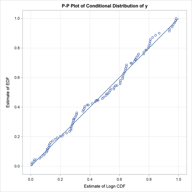
A P-P plot is a scatter plot of the EDF and the CDF estimates. The model for which the points are scattered closer to the unit-slope reference line is a better fit. The P-P plot for the lognormal distribution is shown in Figure 23.10. It indicates that the EDF and the CDF match very closely. In contrast, the P-P plot for the Weibull distribution, also shown in Figure 23.10, indicates a poor fit.
Figure 23.10: P-P Plots for Lognormal and Weibull Models Fitted to Truncated and Censored Data

-
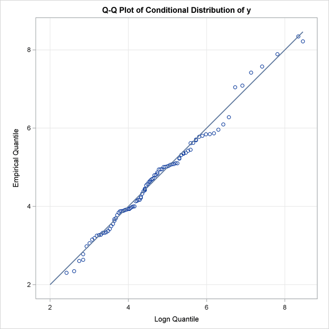
A Q-Q plot is a scatter plot of empirical quantiles and the quantiles of a parametric distribution. Like the P-P plot, points scattered closer to the unit-slope reference line indicate a better fit. The Q-Q plots of lognormal and Weibull distributions are shown in Figure 23.11, which confirm the conclusions arrived at by comparing the P-P plots.
Figure 23.11: Q-Q Plots for Lognormal and Weibull Models Fitted to Truncated and Censored Data

Specifying Initial Values for Parameters
All the predefined distributions have parameter initialization functions built into them. For the current example, Figure 23.12 shows the initial values that are obtained by the predefined method for the Burr distribution. It also shows the summary of the optimization process and the final parameter estimates.
Figure 23.12: Burr Model Summary for the Truncated and Censored Data
| Initial Parameter Values and Bounds for Burr Distribution |
|||
|---|---|---|---|
| Parameter | Initial Value | Lower Bound | Upper Bound |
| Theta | 4.78102 | 1.05367E-8 | Infty |
| Alpha | 2.00000 | 1.05367E-8 | Infty |
| Gamma | 2.00000 | 1.05367E-8 | Infty |
| Optimization Summary for Burr Distribution | |
|---|---|
| Optimization Technique | Trust Region |
| Number of Iterations | 8 |
| Number of Function Evaluations | 23 |
| Log Likelihood | -148.20614 |
| Parameter Estimates for Burr Distribution | ||||
|---|---|---|---|---|
| Parameter | Estimate | Standard Error |
t Value | Approx Pr > |t| |
| Theta | 4.76980 | 0.62492 | 7.63 | <.0001 |
| Alpha | 1.16363 | 0.58859 | 1.98 | 0.0509 |
| Gamma | 5.94081 | 1.05004 | 5.66 | <.0001 |
You can specify a different set of initial values if estimates are available from fitting the distribution to similar data. For this example, the parameters of the Burr distribution can be initialized with the final parameter estimates of the Burr distribution that were obtained in the first example (shown in Figure 23.5). One of the ways in which you can specify the initial values is as follows:
/*------ Specifying initial values using INIT= option -------*/
proc severity data=test_sev2 crit=aicc print=all plots=none;
   loss y / lt=threshold rc=limit;

   dist burr(init=(theta=4.62348 alpha=1.15706 gamma=6.41227));
run;
The names of the parameters specified in the INIT option must match the names used in the definition of the distribution. The results obtained with these initial values are shown in Figure 23.13. These results indicate that new set of initial values causes the optimizer to reach the same solution with fewer iterations and function evaluations as compared to the default initialization.
Figure 23.13: Burr Model Optimization Summary for the Truncated and Censored Data
| Optimization Summary for Burr Distribution | |
|---|---|
| Optimization Technique | Trust Region |
| Number of Iterations | 5 |
| Number of Function Evaluations | 16 |
| Log Likelihood | -148.20614 |
| Parameter Estimates for Burr Distribution | ||||
|---|---|---|---|---|
| Parameter | Estimate | Standard Error |
t Value | Approx Pr > |t| |
| Theta | 4.76980 | 0.62492 | 7.63 | <.0001 |
| Alpha | 1.16363 | 0.58859 | 1.98 | 0.0509 |
| Gamma | 5.94081 | 1.05004 | 5.66 | <.0001 |