The AUTOREG Procedure
- Overview
-
Getting Started

-
Syntax
-
DetailsMissing ValuesAutoregressive Error ModelAlternative Autocorrelation Correction MethodsGARCH ModelsHeteroscedasticity- and Autocorrelation-Consistent Covariance Matrix EstimatorGoodness-of-Fit Measures and Information CriteriaTestingPredicted ValuesOUT= Data SetOUTEST= Data SetPrinted OutputODS Table NamesODS Graphics
-
Examples
- References
Forecasting Autoregressive Error Models
To produce forecasts for future periods, include observations for the forecast periods in the input data set. The forecast observations must provide values for the independent variables and have missing values for the response variable.
For the time trend model, the only regressor is time. The following statements add observations for time periods 37 through 46 to the data set A to produce an augmented data set B:
data b;
   y = .;
   do time = 37 to 46; output; end;
run;

data b;
   merge a b;
   by time;
run;
To produce the forecast, use the augmented data set as input to PROC AUTOREG, and specify the appropriate options in the OUTPUT statement. The following statements produce forecasts for the time trend with autoregressive error model. The output data set includes all the variables in the input data set, the forecast values (YHAT), the predicted trend (YTREND), and the upper (UCL) and lower (LCL) 95% confidence limits.
proc autoreg data=b;
   model y = time / nlag=2 method=ml;
   output out=p p=yhat pm=ytrend
                lcl=lcl ucl=ucl;
run;
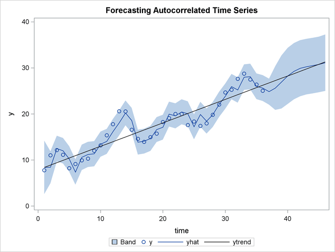
The following statements plot the predicted values and confidence limits, and they also plot the trend line for reference. The actual observations are shown for periods 16 through 36, and a reference line is drawn at the start of the out-of-sample forecasts.
title 'Forecasting Autocorrelated Time Series';
proc sgplot data=p;
   band x=time upper=ucl lower=lcl;
   scatter x=time y=y;
   series x=time y=yhat;
   series x=time y=ytrend / lineattrs=(color=black);
run;
The plot is shown in Figure 8.6. Notice that the forecasts take into account the recent departures from the trend but converge back to the trend line for longer forecast horizons.
Figure 8.6: PROC AUTOREG Forecasts