The ARIMA Procedure
- Overview
-
Getting Started
 The Three Stages of ARIMA Modeling Identification Stage Estimation and Diagnostic Checking Stage Forecasting Stage Using ARIMA Procedure Statements General Notation for ARIMA Models Stationarity Differencing Subset, Seasonal, and Factored ARMA Models Input Variables and Regression with ARMA Errors Intervention Models and Interrupted Time Series Rational Transfer Functions and Distributed Lag Models Forecasting with Input Variables Data Requirements
 -
Syntax
-
Details
The Inverse Autocorrelation Function The Partial Autocorrelation Function The Cross-Correlation Function The ESACF Method The MINIC Method The SCAN Method Stationarity Tests Prewhitening Identifying Transfer Function Models Missing Values and Autocorrelations Estimation Details Specifying Inputs and Transfer Functions Initial Values Stationarity and Invertibility Naming of Model Parameters Missing Values and Estimation and Forecasting Forecasting Details Forecasting Log Transformed Data Specifying Series Periodicity Detecting Outliers OUT= Data Set OUTCOV= Data Set OUTEST= Data Set OUTMODEL= SAS Data Set OUTSTAT= Data Set Printed Output ODS Table Names Statistical Graphics
-
Examples
- References
| Detecting Outliers |
You can use the OUTLIER statement to detect changes in the level of the response series that are not accounted for by the estimated model. The types of changes considered are additive outliers (AO), level shifts (LS), and temporary changes (TC).
Let  be a regression variable that describes some type of change in the mean response. In time series literature is called a shock signature. An additive outlier at some time point
  corresponds to a shock signature such that
  and is 0.0 at all other points. Similarly a permanent level shift that originates at time has a shock signature such that is 0.0 for
  and 1.0 for
  . A temporary level shift of duration
  that originates at time has equal to 1.0 between and
  and 0.0 otherwise.
Suppose that you are estimating the ARIMA model
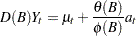 |
where  is the response series,
  is the differencing polynomial in the backward shift operator B (possibly identity),
  is the transfer function input,
  and
and  are the AR and MA polynomials, respectively, and
  is the Gaussian white noise series.
The problem of detection of level shifts in the OUTLIER statement is formulated as a problem of sequential selection of shock signatures that improve the model in the ESTIMATE statement. This is similar to the forward selection process in the stepwise regression procedure. The selection process starts with considering shock signatures of the type specified in the TYPE= option, originating at each nonmissing measurement. This involves testing  versus
  in the model
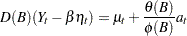 |
for each of these shock signatures. The most significant shock signature, if it also satisfies the significance criterion in ALPHA= option, is included in the model. If no significant shock signature is found, then the outlier detection process stops; otherwise this augmented model, which incorporates the selected shock signature in its transfer function input, becomes the null model for the subsequent selection process. This iterative process stops if at any stage no more significant shock signatures are found or if the number of iterations exceeds the maximum search number that results due to the MAXNUM= and MAXPCT= settings. In all these iterations, the parameters of the ARIMA model in the ESTIMATE statement are held fixed.
The precise details of the testing procedure for a given shock signature are as follows:
The preceding testing problem is equivalent to testing versus in the following "regression with ARMA errors" model
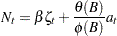 |
where 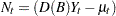 is the "noise" process and
  is the "effective" shock signature.
In this setting, under 
 is a mean zero Gaussian vector with variance covariance matrix
  . Here
  is the variance of the white noise process and
  is the variance-covariance matrix associated with the ARMA model. Moreover, under
  ,
,  has
has  as the mean vector where
  . Additionally, the generalized least squares estimate of
  and its variance is given by
 |
 |
 |
|||
 |
|
 |
where  and
and  . The test statistic
  is used to test the significance of , which has an approximate chi-squared distribution with 1 degree of freedom under
  . The type of estimate of
  used in the calculation of
  can be specified by the SIGMA= option. The default setting is SIGMA=ROBUST, which corresponds to a robust estimate suggested in an outlier detection procedure in X-12-ARIMA, the Census Bureau’s time series analysis program; see Findley et al. (1998) for additional information. The robust estimate of is computed by the formula
 |
where  are the standardized residuals of the null ARIMA model. The setting SIGMA=MSE corresponds to the usual mean squared error estimate (MSE) computed the same way as in the ESTIMATE statement with the NODF option.
The quantities  and
and  are efficiently computed by a method described in de Jong and Penzer (1998); see also Kohn and Ansley (1985).
Modeling in the Presence of Outliers
In practice, modeling and forecasting time series data in the presence of outliers is a difficult problem for several reasons. The presence of outliers can adversely affect the model identification and estimation steps. Their presence close to the end of the observation period can have a serious impact on the forecasting performance of the model. In some cases, level shifts are associated with changes in the mechanism that drives the observation process, and separate models might be appropriate to different sections of the data. In view of all these difficulties, diagnostic tools such as outlier detection and residual analysis are essential in any modeling process.
The following modeling strategy, which incorporates level shift detection in the familiar Box-Jenkins modeling methodology, seems to work in many cases:
Proceed with model identification and estimation as usual. Suppose this results in a tentative ARIMA model, say M.
Check for additive and permanent level shifts unaccounted for by the model M by using the OUTLIER statement. In this step, unless there is evidence to justify it, the number of level shifts searched should be kept small.
Augment the original dataset with the regression variables that correspond to the detected outliers.
Include the first few of these regression variables in M, and call this model M1. Reestimate all the parameters of M1. It is important not to include too many of these outlier variables in the model in order to avoid the danger of over-fitting.
Check the adequacy of M1 by examining the parameter estimates, residual analysis, and outlier detection. Refine it more if necessary.