| The VARMAX Procedure |
Example 32.1 Analysis of U.S. Economic Variables
Consider the following four-dimensional system of U.S. economic variables. Quarterly data for the years 1954 to 1987 are used (Lütkepohl 1993, Table E.3.).
title 'Analysis of U.S. Economic Variables';
data us_money;
   date=intnx( 'qtr', '01jan54'd, _n_-1 );
   format date yyq. ;
   input y1 y2 y3 y4 @@;
   y1=log(y1);
   y2=log(y2);
   label y1='log(real money stock M1)'
         y2='log(GNP in bil. of 1982 dollars)'
         y3='Discount rate on 91-day T-bills'
         y4='Yield on 20-year Treasury bonds';
datalines;
450.9 1406.8  0.010800000 0.026133333
453.0 1401.2 0.0081333333 0.025233333

   ... more lines ...
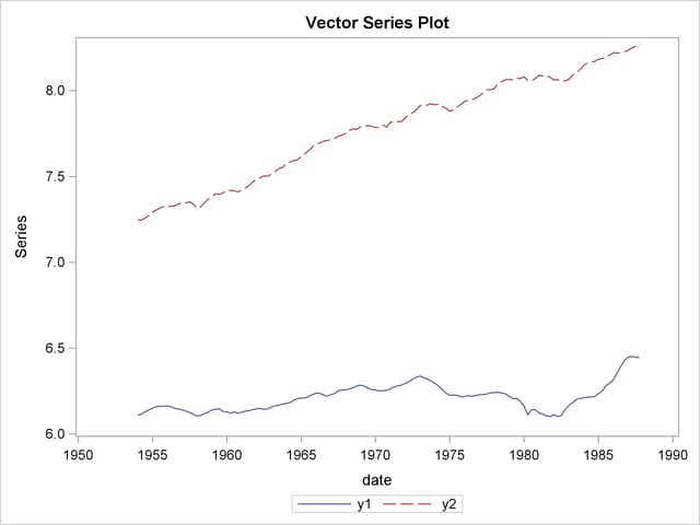
The following statements plot the series and proceed with the VARMAX procedure.
proc timeseries data=us_money vectorplot=series;
   id date interval=qtr;
   var y1 y2;
run;
Output 32.1.1 shows the plot of the variables  and
and  .
.
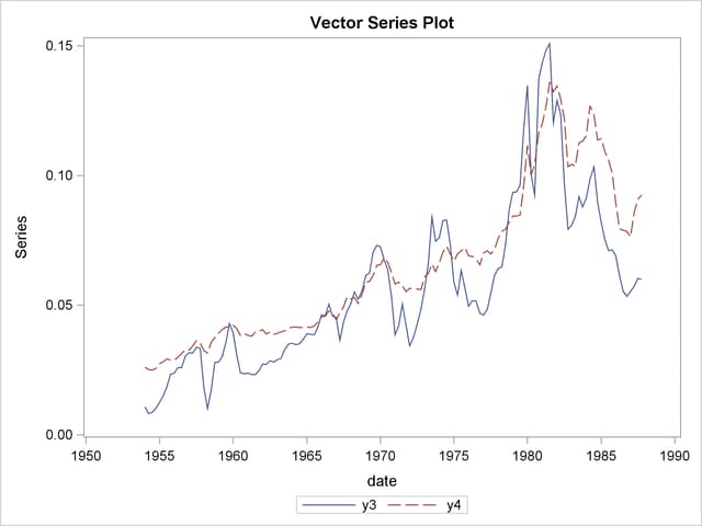
The following statements plot the variables  and
and  .
.
proc timeseries data=us_money vectorplot=series;
   id date interval=qtr;
   var y3 y4;
run;
Output 32.1.2 shows the plot of the variables and .
proc varmax data=us_money;
   id date interval=qtr;
   model y1-y4 / p=2 lagmax=6 dftest
                 print=(iarr(3) estimates diagnose)
                 cointtest=(johansen=(iorder=2))
                 ecm=(rank=1 normalize=y1);
   cointeg rank=1 normalize=y1 exogeneity;
run;
This example performs the Dickey-Fuller test for stationarity, the Johansen cointegrated test integrated order 2, and the exogeneity test. The VECM(2) is fit to the data. From the outputs shown in Output 32.1.5, you can see that the series has unit roots and is cointegrated in rank 1 with integrated order 1. The fitted VECM(2) is given as
The


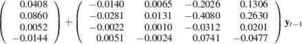

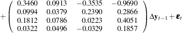
 prefixed to a variable name implies differencing.
Output 32.1.3 through Output 32.1.14 show the details. Output 32.1.3 shows the descriptive statistics.
| Number of Observations | 136 |
|---|---|
| Number of Pairwise Missing | 0 |
| Simple Summary Statistics | |||||||
|---|---|---|---|---|---|---|---|
| Variable | Type | N | Mean | Standard Deviation |
Min | Max | Label |
| y1 | Dependent | 136 | 6.21295 | 0.07924 | 6.10278 | 6.45331 | log(real money stock M1) |
| y2 | Dependent | 136 | 7.77890 | 0.30110 | 7.24508 | 8.27461 | log(GNP in bil. of 1982 dollars) |
| y3 | Dependent | 136 | 0.05608 | 0.03109 | 0.00813 | 0.15087 | Discount rate on 91-day T-bills |
| y4 | Dependent | 136 | 0.06458 | 0.02927 | 0.02490 | 0.13600 | Yield on 20-year Treasury bonds |
Output 32.1.4 shows the output for Dickey-Fuller tests for the nonstationarity of each series. The null hypotheses is to test a unit root. All series have a unit root.
| Unit Root Test | |||||
|---|---|---|---|---|---|
| Variable | Type | Rho | Pr < Rho | Tau | Pr < Tau |
| y1 | Zero Mean | 0.05 | 0.6934 | 1.14 | 0.9343 |
| Single Mean | -2.97 | 0.6572 | -0.76 | 0.8260 | |
| Trend | -5.91 | 0.7454 | -1.34 | 0.8725 | |
| y2 | Zero Mean | 0.13 | 0.7124 | 5.14 | 0.9999 |
| Single Mean | -0.43 | 0.9309 | -0.79 | 0.8176 | |
| Trend | -9.21 | 0.4787 | -2.16 | 0.5063 | |
| y3 | Zero Mean | -1.28 | 0.4255 | -0.69 | 0.4182 |
| Single Mean | -8.86 | 0.1700 | -2.27 | 0.1842 | |
| Trend | -18.97 | 0.0742 | -2.86 | 0.1803 | |
| y4 | Zero Mean | 0.40 | 0.7803 | 0.45 | 0.8100 |
| Single Mean | -2.79 | 0.6790 | -1.29 | 0.6328 | |
| Trend | -12.12 | 0.2923 | -2.33 | 0.4170 | |
The Johansen cointegration rank test shows whether the series is integrated order either 1 or 2 as shown in Output 32.1.5. The last two columns in Output 32.1.5 explain the cointegration rank test with integrated order 1. The results indicate that there is the cointegrated relationship with the cointegration rank 1 with respect to the 0.05 significance level because the test statistic of 20.6542 is smaller than the critical value of 29.38. Now, look at the row associated with  . Compare the test statistic value and critical value pairs such as (219.62395, 29.38), (89.21508, 15.34), and (27.32609, 3.84). There is no evidence that the series are integrated order 2 at the 0.05 significance level.
Output 32.1.6 shows the estimates of the long-run parameter,  , and the adjustment coefficient,
  .
.
| Beta | ||||
|---|---|---|---|---|
| Variable | 1 | 2 | 3 | 4 |
| y1 | 1.00000 | 1.00000 | 1.00000 | 1.00000 |
| y2 | -0.46458 | -0.63174 | -0.69996 | -0.16140 |
| y3 | 14.51619 | -1.29864 | 1.37007 | -0.61806 |
| y4 | -9.35520 | 7.53672 | 2.47901 | 1.43731 |
| Alpha | ||||
|---|---|---|---|---|
| Variable | 1 | 2 | 3 | 4 |
| y1 | -0.01396 | 0.01396 | -0.01119 | 0.00008 |
| y2 | -0.02811 | -0.02739 | -0.00032 | 0.00076 |
| y3 | -0.00215 | -0.04967 | -0.00183 | -0.00072 |
| y4 | 0.00510 | -0.02514 | -0.00220 | 0.00016 |
Output 32.1.7 shows the estimates  and
and  .
.
| Eta | ||||
|---|---|---|---|---|
| Variable | 1 | 2 | 3 | 4 |
| y1 | 52.74907 | 41.74502 | -20.80403 | 55.77415 |
| y2 | -49.10609 | -9.40081 | 98.87199 | 22.56416 |
| y3 | 68.29674 | -144.83173 | -27.35953 | 15.51142 |
| y4 | 121.25932 | 271.80496 | 85.85156 | -130.11599 |
| Xi | ||||
|---|---|---|---|---|
| Variable | 1 | 2 | 3 | 4 |
| y1 | -0.00842 | -0.00052 | -0.00208 | -0.00250 |
| y2 | 0.00141 | 0.00213 | -0.00736 | -0.00058 |
| y3 | -0.00445 | 0.00541 | -0.00150 | 0.00310 |
| y4 | -0.00211 | -0.00064 | -0.00130 | 0.00197 |
Output 32.1.8 shows that the VECM(2) is fit to the data. The ECM=(RANK=1) option produces the estimates of the long-run parameter, , and the adjustment coefficient, .
| Type of Model | VECM(2) |
|---|---|
| Estimation Method | Maximum Likelihood Estimation |
| Cointegrated Rank | 1 |
| Beta | |
|---|---|
| Variable | 1 |
| y1 | 1.00000 |
| y2 | -0.46458 |
| y3 | 14.51619 |
| y4 | -9.35520 |
| Alpha | |
|---|---|
| Variable | 1 |
| y1 | -0.01396 |
| y2 | -0.02811 |
| y3 | -0.00215 |
| y4 | 0.00510 |
Output 32.1.9 shows the parameter estimates in terms of the constant, the lag one coefficients ( ) contained in the
  estimates, and the coefficients associated with the lag one first differences (
 ).
).
| Constant | |
|---|---|
| Variable | Constant |
| y1 | 0.04076 |
| y2 | 0.08595 |
| y3 | 0.00518 |
| y4 | -0.01438 |
| Parameter Alpha * Beta' Estimates | ||||
|---|---|---|---|---|
| Variable | y1 | y2 | y3 | y4 |
| y1 | -0.01396 | 0.00648 | -0.20263 | 0.13059 |
| y2 | -0.02811 | 0.01306 | -0.40799 | 0.26294 |
| y3 | -0.00215 | 0.00100 | -0.03121 | 0.02011 |
| y4 | 0.00510 | -0.00237 | 0.07407 | -0.04774 |
| AR Coefficients of Differenced Lag | |||||
|---|---|---|---|---|---|
| DIF Lag | Variable | y1 | y2 | y3 | y4 |
| 1 | y1 | 0.34603 | 0.09131 | -0.35351 | -0.96895 |
| y2 | 0.09936 | 0.03791 | 0.23900 | 0.28661 | |
| y3 | 0.18118 | 0.07859 | 0.02234 | 0.40508 | |
| y4 | 0.03222 | 0.04961 | -0.03292 | 0.18568 | |
Output 32.1.10 shows the parameter estimates and their significance.
| Model Parameter Estimates | ||||||
|---|---|---|---|---|---|---|
| Equation | Parameter | Estimate | Standard Error |
t Value | Pr > |t| | Variable |
| D_y1 | CONST1 | 0.04076 | 0.01418 | 2.87 | 0.0048 | 1 |
| AR1_1_1 | -0.01396 | 0.00495 | y1(t-1) | |||
| AR1_1_2 | 0.00648 | 0.00230 | y2(t-1) | |||
| AR1_1_3 | -0.20263 | 0.07191 | y3(t-1) | |||
| AR1_1_4 | 0.13059 | 0.04634 | y4(t-1) | |||
| AR2_1_1 | 0.34603 | 0.06414 | 5.39 | 0.0001 | D_y1(t-1) | |
| AR2_1_2 | 0.09131 | 0.07334 | 1.25 | 0.2154 | D_y2(t-1) | |
| AR2_1_3 | -0.35351 | 0.11024 | -3.21 | 0.0017 | D_y3(t-1) | |
| AR2_1_4 | -0.96895 | 0.20737 | -4.67 | 0.0001 | D_y4(t-1) | |
| D_y2 | CONST2 | 0.08595 | 0.01679 | 5.12 | 0.0001 | 1 |
| AR1_2_1 | -0.02811 | 0.00586 | y1(t-1) | |||
| AR1_2_2 | 0.01306 | 0.00272 | y2(t-1) | |||
| AR1_2_3 | -0.40799 | 0.08514 | y3(t-1) | |||
| AR1_2_4 | 0.26294 | 0.05487 | y4(t-1) | |||
| AR2_2_1 | 0.09936 | 0.07594 | 1.31 | 0.1932 | D_y1(t-1) | |
| AR2_2_2 | 0.03791 | 0.08683 | 0.44 | 0.6632 | D_y2(t-1) | |
| AR2_2_3 | 0.23900 | 0.13052 | 1.83 | 0.0695 | D_y3(t-1) | |
| AR2_2_4 | 0.28661 | 0.24552 | 1.17 | 0.2453 | D_y4(t-1) | |
| D_y3 | CONST3 | 0.00518 | 0.01608 | 0.32 | 0.7476 | 1 |
| AR1_3_1 | -0.00215 | 0.00562 | y1(t-1) | |||
| AR1_3_2 | 0.00100 | 0.00261 | y2(t-1) | |||
| AR1_3_3 | -0.03121 | 0.08151 | y3(t-1) | |||
| AR1_3_4 | 0.02011 | 0.05253 | y4(t-1) | |||
| AR2_3_1 | 0.18118 | 0.07271 | 2.49 | 0.0140 | D_y1(t-1) | |
| AR2_3_2 | 0.07859 | 0.08313 | 0.95 | 0.3463 | D_y2(t-1) | |
| AR2_3_3 | 0.02234 | 0.12496 | 0.18 | 0.8584 | D_y3(t-1) | |
| AR2_3_4 | 0.40508 | 0.23506 | 1.72 | 0.0873 | D_y4(t-1) | |
| D_y4 | CONST4 | -0.01438 | 0.00803 | -1.79 | 0.0758 | 1 |
| AR1_4_1 | 0.00510 | 0.00281 | y1(t-1) | |||
| AR1_4_2 | -0.00237 | 0.00130 | y2(t-1) | |||
| AR1_4_3 | 0.07407 | 0.04072 | y3(t-1) | |||
| AR1_4_4 | -0.04774 | 0.02624 | y4(t-1) | |||
| AR2_4_1 | 0.03222 | 0.03632 | 0.89 | 0.3768 | D_y1(t-1) | |
| AR2_4_2 | 0.04961 | 0.04153 | 1.19 | 0.2345 | D_y2(t-1) | |
| AR2_4_3 | -0.03292 | 0.06243 | -0.53 | 0.5990 | D_y3(t-1) | |
| AR2_4_4 | 0.18568 | 0.11744 | 1.58 | 0.1164 | D_y4(t-1) | |
Output 32.1.11 shows the innovation covariance matrix estimates, the various information criteria results, and the tests for white noise residuals. The residuals have significant correlations at lag 2 and 3. The Portmanteau test results into significant. These results show that a VECM(3) model might be better fit than the VECM(2) model is.
| Covariances of Innovations | ||||
|---|---|---|---|---|
| Variable | y1 | y2 | y3 | y4 |
| y1 | 0.00005 | 0.00001 | -0.00001 | -0.00000 |
| y2 | 0.00001 | 0.00007 | 0.00002 | 0.00001 |
| y3 | -0.00001 | 0.00002 | 0.00007 | 0.00002 |
| y4 | -0.00000 | 0.00001 | 0.00002 | 0.00002 |
| Information Criteria | |
|---|---|
| AICC | -40.6284 |
| HQC | -40.4343 |
| AIC | -40.6452 |
| SBC | -40.1262 |
| FPEC | 2.23E-18 |
| Schematic Representation of Cross Correlations of Residuals |
|||||||
|---|---|---|---|---|---|---|---|
| Variable/Lag | 0 | 1 | 2 | 3 | 4 | 5 | 6 |
| y1 | ++.. | .... | ++.. | .... | +... | ..-- | .... |
| y2 | ++++ | .... | .... | .... | .... | .... | .... |
| y3 | .+++ | .... | +.-. | ..++ | -... | .... | .... |
| y4 | .+++ | .... | .... | ..+. | .... | .... | .... |
| + is > 2*std error, - is < -2*std error, . is between | |||||||
| Portmanteau Test for Cross Correlations of Residuals |
|||
|---|---|---|---|
| Up To Lag | DF | Chi-Square | Pr > ChiSq |
| 3 | 16 | 53.90 | <.0001 |
| 4 | 32 | 74.03 | <.0001 |
| 5 | 48 | 103.08 | <.0001 |
| 6 | 64 | 116.94 | <.0001 |
Output 32.1.12 describes how well each univariate equation fits the data. The residuals for and are off from the normality. Except the residuals for , there are no AR effects on other residuals. Except the residuals for , there are no ARCH effects on other residuals.
| Univariate Model ANOVA Diagnostics | ||||
|---|---|---|---|---|
| Variable | R-Square | Standard Deviation |
F Value | Pr > F |
| y1 | 0.6754 | 0.00712 | 32.51 | <.0001 |
| y2 | 0.3070 | 0.00843 | 6.92 | <.0001 |
| y3 | 0.1328 | 0.00807 | 2.39 | 0.0196 |
| y4 | 0.0831 | 0.00403 | 1.42 | 0.1963 |
| Univariate Model White Noise Diagnostics | |||||
|---|---|---|---|---|---|
| Variable | Durbin Watson |
Normality | ARCH | ||
| Chi-Square | Pr > ChiSq | F Value | Pr > F | ||
| y1 | 2.13418 | 7.19 | 0.0275 | 1.62 | 0.2053 |
| y2 | 2.04003 | 1.20 | 0.5483 | 1.23 | 0.2697 |
| y3 | 1.86892 | 253.76 | <.0001 | 1.78 | 0.1847 |
| y4 | 1.98440 | 105.21 | <.0001 | 21.01 | <.0001 |
| Univariate Model AR Diagnostics | ||||||||
|---|---|---|---|---|---|---|---|---|
| Variable | AR1 | AR2 | AR3 | AR4 | ||||
| F Value | Pr > F | F Value | Pr > F | F Value | Pr > F | F Value | Pr > F | |
| y1 | 0.68 | 0.4126 | 2.98 | 0.0542 | 2.01 | 0.1154 | 2.48 | 0.0473 |
| y2 | 0.05 | 0.8185 | 0.12 | 0.8842 | 0.41 | 0.7453 | 0.30 | 0.8762 |
| y3 | 0.56 | 0.4547 | 2.86 | 0.0610 | 4.83 | 0.0032 | 3.71 | 0.0069 |
| y4 | 0.01 | 0.9340 | 0.16 | 0.8559 | 1.21 | 0.3103 | 0.95 | 0.4358 |
The PRINT=(IARR) option provides the VAR(2) representation in Output 32.1.13.
| Infinite Order AR Representation | |||||
|---|---|---|---|---|---|
| Lag | Variable | y1 | y2 | y3 | y4 |
| 1 | y1 | 1.33208 | 0.09780 | -0.55614 | -0.83836 |
| y2 | 0.07125 | 1.05096 | -0.16899 | 0.54955 | |
| y3 | 0.17903 | 0.07959 | 0.99113 | 0.42520 | |
| y4 | 0.03732 | 0.04724 | 0.04116 | 1.13795 | |
| 2 | y1 | -0.34603 | -0.09131 | 0.35351 | 0.96895 |
| y2 | -0.09936 | -0.03791 | -0.23900 | -0.28661 | |
| y3 | -0.18118 | -0.07859 | -0.02234 | -0.40508 | |
| y4 | -0.03222 | -0.04961 | 0.03292 | -0.18568 | |
| 3 | y1 | 0.00000 | 0.00000 | 0.00000 | 0.00000 |
| y2 | 0.00000 | 0.00000 | 0.00000 | 0.00000 | |
| y3 | 0.00000 | 0.00000 | 0.00000 | 0.00000 | |
| y4 | 0.00000 | 0.00000 | 0.00000 | 0.00000 | |
Output 32.1.14 shows whether each variable is the weak exogeneity of other variables. The variable is not the weak exogeneity of other variables, , , and ; the variable is not the weak exogeneity of other variables, , , and ; the variable and are the weak exogeneity of other variables.
Copyright © SAS Institute, Inc. All Rights Reserved.