| The UCM Procedure |
Example 31.2 Variable Star Data
The series in this example is studied in detail in Bloomfield (2000). This series consists of brightness measurements (magnitude) of a variable star taken at midnight for 600 consecutive days. The data can be downloaded from a time series archive maintained by the University of York, England (http://www.york.ac.uk/depts/maths/data/ts/welcome.htm (series number 26)). The following DATA step statements read the data in a SAS data set.
data star;
   input magnitude @@;
   day = _n_;
datalines;
  25  28  31  32  33  33  32  31  28   25   22   18
  14  10   7   4   2   0   0   0   2    4    8   11
  15  19  23  26  29  32  33  34  33   32   30   27
  24  20  17  13  10   7   5   3   3    3    4    5
   7  10  13  16  19  22  24  26  27   28   29   28
  27  25  24  21  19  17  15  13  12   11   11   10

   ... more lines ...
The following statements use the TIMESERIES procedure to get a timeseries plot of the series (see Output 31.2.1).
ods graphics on;
proc timeseries data=star plot=series;
   var magnitude;
run;
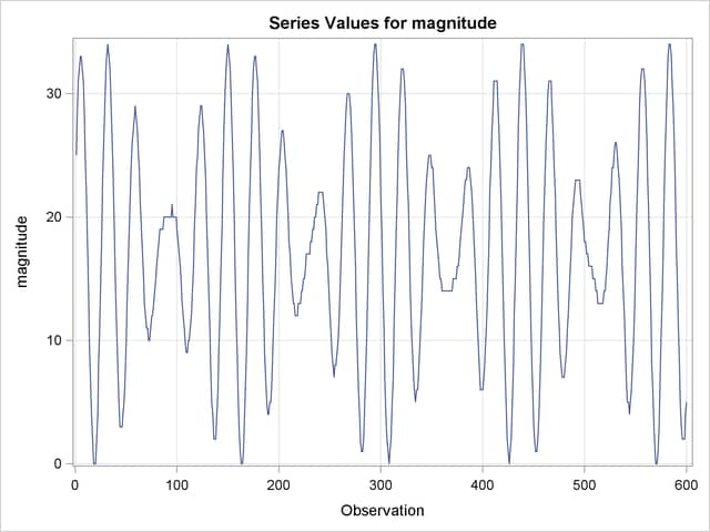
The plot clearly shows the cyclic nature of the series. Bloomfield shows that the series is very well explained by a model that includes two deterministic cycles that have periods 29.0003 and 24.0001 days, a constant term, and a simple error term. He also mentions the difficulty involved in estimating the periods from the data (see Bloomfield 2000, Chapter 3). In his case the cycle periods are estimated by least squares, and the sum of squares surface has multiple local optima and ridges. The following statements show how to use the UCM procedure to fit this two-cycle model to the series. The constant term in the model is specified by holding the variance parameter of the level component to zero.
proc ucm data=star;
   model magnitude;
   irregular;
   level var=0 noest;
   cycle;
   cycle;
   estimate;
run;
The final parameter estimates and the goodness-of-fit statistics are shown in Output 31.2.2 and Output 31.2.3, respectively. The model fit appears to be good.
| Final Estimates of the Free Parameters | |||||
|---|---|---|---|---|---|
| Component | Parameter | Estimate | Approx Std Error |
t Value | Approx Pr > |t| |
| Irregular | Error Variance | 0.09257 | 0.0053845 | 17.19 | <.0001 |
| Cycle_1 | Damping Factor | 1.00000 | 1.81175E-7 | 5519514 | <.0001 |
| Cycle_1 | Period | 29.00036 | 0.0022709 | 12770.4 | <.0001 |
| Cycle_1 | Error Variance | 0.00000882 | 5.27213E-6 | 1.67 | 0.0944 |
| Cycle_2 | Damping Factor | 1.00000 | 2.11939E-7 | 4718334 | <.0001 |
| Cycle_2 | Period | 24.00011 | 0.0019128 | 12547.2 | <.0001 |
| Cycle_2 | Error Variance | 0.00000535 | 3.56374E-6 | 1.50 | 0.1330 |
| Fit Statistics Based on Residuals | |
|---|---|
| Mean Squared Error | 0.12072 |
| Root Mean Squared Error | 0.34745 |
| Mean Absolute Percentage Error | 2.65141 |
| Maximum Percent Error | 36.38991 |
| R-Square | 0.99850 |
| Adjusted R-Square | 0.99849 |
| Random Walk R-Square | 0.97281 |
| Amemiya's Adjusted R-Square | 0.99847 |
| Number of non-missing residuals used for computing the fit statistics = 599 | |
A summary of the cycles in the model is given in Output 31.2.4.
Note that the estimated periods are the same as in Bloomfield’s model, the damping factors are nearly equal to 1.0, and the disturbance variances are very close to zero, implying persistent deterministic cycles. In fact, this model is identical to Bloomfield’s model.
Copyright © SAS Institute, Inc. All Rights Reserved.