| The TIMEID Procedure |
Example 28.1 Examining a Weekly Time ID Variable
This example illustrates how problems in a weekly time series can be visualized and quantified using the TIMEID procedure’s diagnostic capabilities.
The following DATA step creates a data set that contains time values spaced in three week intervals where some weeks have been skipped or duplicated and some have been recorded on different weekdays.
data triweek;
   format date date.;
   input date : date. @@;
datalines;
28DEC48 18JAN49 08FEB49 01MAR49 22MAR49 12APR49 03MAY49 24MAY49
17JUN49 05JUL49 26JUL49 16AUG49 06SEP49 27SEP49 18OCT49 08NOV49

   ... more lines ...
The following TIMEID procedure statements generate an ODS display of the time series that characterizes interval counts, offsets, and spans in the time ID variable.
proc timeid data=triweek print=all plot=all;
  id date interval=week3;
run;
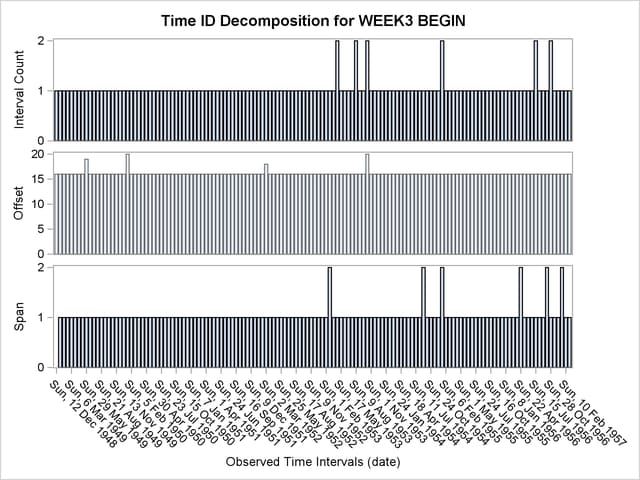
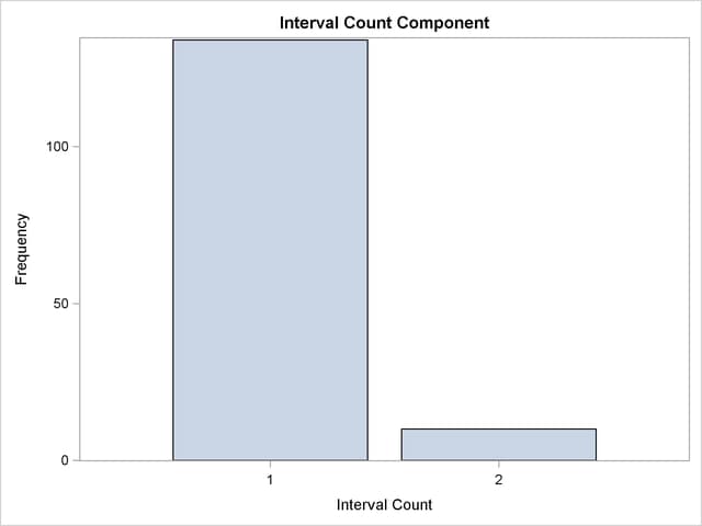
The Time ID decomposition listing and plot shown in Output 28.1.1 and Output 28.1.2 summarize how well the WEEK3 interval fits the time ID values by showing the number of counts, offsets, and spans for each time interval that is represented by the DATE variable. The listing in Output 28.1.1 has been truncated to include only the first 10 observations. The Time ID plots in Output 28.1.2 indicate that there are duplicated time ID values for a three-week time interval in the Counts plot. The duplicated time intervals have a Count value of 2. The Offsets plot shows which days in the 21 day cycle have been used to record each time interval in the series. The Spans plot records values of 2 for six time intervals where no observations were recorded in the previous interval. The three component plots are histogram summaries of the diagnostic quantities plotted against individual intervals in the decomposition plots. The component plots can be useful in diagnosing time series that contain many time intervals.
| Time Component | ||||
|---|---|---|---|---|
| Value Index |
date | Offset | Span | Interval Count |
| 1 | Sun, 12 Dec 1948 | 16 | . | 1 |
| 2 | Sun, 2 Jan 1949 | 16 | 1 | 1 |
| 3 | Sun, 23 Jan 1949 | 16 | 1 | 1 |
| 4 | Sun, 13 Feb 1949 | 16 | 1 | 1 |
| 5 | Sun, 6 Mar 1949 | 16 | 1 | 1 |
| 6 | Sun, 27 Mar 1949 | 16 | 1 | 1 |
| 7 | Sun, 17 Apr 1949 | 16 | 1 | 1 |
| 8 | Sun, 8 May 1949 | 16 | 1 | 1 |
| 9 | Sun, 29 May 1949 | 19 | 1 | 1 |
| 10 | Sun, 19 Jun 1949 | 16 | 1 | 1 |
Output 28.1.3 and Output 28.1.4 describe the distribution of counts of duplicated WEEK3 intervals in the TriWeek data set. For this data set there are 134 intervals that contain one DATE value, and 10 intervals that contain two DATE values.
| Component | |||
|---|---|---|---|
| Value Index |
Interval Count |
Frequency | Percentage |
| 1 | 1 | 134 | 93.055556 |
| 2 | 2 | 10 | 6.944444 |
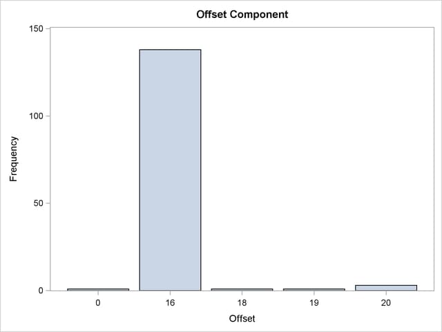
The offsets diagnostics Output 28.1.5 and Output 28.1.6 show the distribution of days in the 21-day WEEK3 interval used to record the time intervals in the series. The observations in the TriWeek data set represent intervals with five different offsets from the beginning of the WEEK3 interval: 0, 16, 18, 19 and 20. The high prevalence of intervals with offset 16 indicates that the TriWeek data set would be represented better using the WEEK3.17 interval.
| Component | |||
|---|---|---|---|
| Value Index |
Offset | Frequency | Percentage |
| 1 | 0 | 1 | 0.694444 |
| 2 | 16 | 138 | 95.833333 |
| 3 | 18 | 1 | 0.694444 |
| 4 | 19 | 1 | 0.694444 |
| 5 | 20 | 3 | 2.083333 |
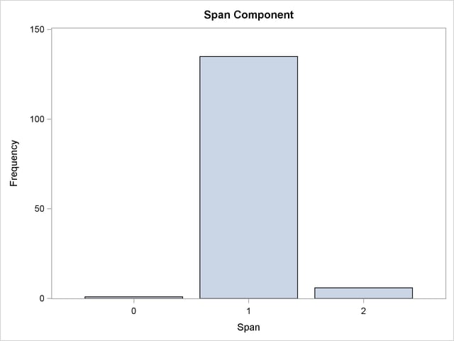
The span diagnostics Output 28.1.7 and Output 28.1.8 show the distribution of the span sizes between successive DATE values. The TriWeek data set has three different span sizes of widths 0, 1 and 2. Here one span corresponds to the width of a WEEK3 interval.
| Component | |||
|---|---|---|---|
| Value Index |
Span | Frequency | Percentage |
| 1 | 0 | 1 | 0.704225 |
| 2 | 1 | 135 | 95.070423 |
| 3 | 2 | 6 | 4.225352 |
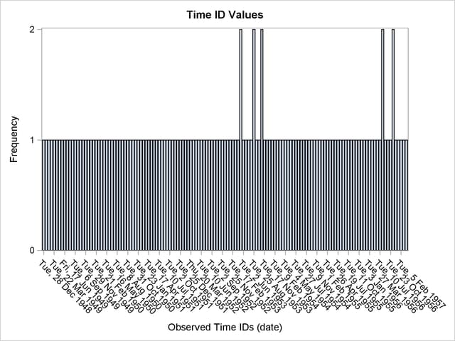
Output 28.1.9 and Output 28.1.10 show the distribution of time ID values before alignment to the WEEK3 interval. The listing in Output 28.1.9 has been truncated to include only the first 10 observations.
| Time ID Values for DATE | |||
|---|---|---|---|
| Value Index |
date | Frequency | Percentage |
| 1 | Tue, 28 Dec 1948 | 1 | 0.694444 |
| 2 | Tue, 18 Jan 1949 | 1 | 0.694444 |
| 3 | Tue, 8 Feb 1949 | 1 | 0.694444 |
| 4 | Tue, 1 Mar 1949 | 1 | 0.694444 |
| 5 | Tue, 22 Mar 1949 | 1 | 0.694444 |
| 6 | Tue, 12 Apr 1949 | 1 | 0.694444 |
| 7 | Tue, 3 May 1949 | 1 | 0.694444 |
| 8 | Tue, 24 May 1949 | 1 | 0.694444 |
| 9 | Fri, 17 Jun 1949 | 1 | 0.694444 |
| 10 | Tue, 5 Jul 1949 | 1 | 0.694444 |
Copyright © SAS Institute, Inc. All Rights Reserved.