| The SEVERITY Procedure |
| Predefined Distribution Models |
A set of predefined distribution models is provided with the SEVERITY procedure. A summary of the models is provided in Table 22.3. For each distribution model, the table lists the parameters in the order in which they appear in the signature of the functions or subroutines that accept distribution parameters as input or output arguments. The table also mentions the bounds on the parameters. If the bounds are different from their default values, then the distribution model contains appropriately defined name_LOWERBOUNDS or name_UPPERBOUNDS subroutines.
All the predefined distribution models, except LOGN, are parameterized such that their first parameter is the scale parameter. For LOGN, the first parameter  is a log-transformed scale parameter, which is specified by using the LOGN_SCALETRANSFORM subroutine. The presence of scale parameter enables you to use any of the predefined distributions as a candidate for estimating regression effects.
If you need to use the functions or subroutines defined in the predefined distributions in SAS statements other than the PROC SEVERITY step (such as in a DATA step), then they are available to you in the SASHELP.SVRTDIST library. Specify the library by using the OPTIONS global statement to set the CMPLIB= system option prior to using these functions. Note that you do not need to use the CMPLIB= option in order to use the predefined distributions with PROC SEVERITY.
Name |
Distribution |
Parameters |
PDF ( |
|
|---|---|---|---|---|
BURR |
Burr |
|
|
|
|
|
|
||
EXP |
Exponential |
|
|
|
|
|
|||
GAMMA |
Gamma |
|
|
|
|
|
|||
GPD |
Generalized |
|
|
|
Pareto |
|
|
||
IGAUSS |
Inverse Gaussian |
|
|
|
(Wald) |
|
|
||
|
||||
LOGN |
Lognormal |
|
|
|
|
|
|
||
PARETO |
Pareto |
|
|
|
|
|
|||
WEIBULL |
Weibull |
|
|
|
|
|
|||
Notes: |
||||
1. |
||||
2. |
||||
3. Parameters are listed in the order in which they are defined in the distribution model. |
||||
4. |
||||
5. |
||||
 ) and CDF (
 )
)  ,
, 


 , wherever
  is used.
 .
. is the lower incomplete gamma function.
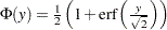 is the standard normal CDF.
Parameter Initialization for Predefined Distribution Models
The definition of each distribution model also contains a name_PARMINIT subroutine to initialize the parameters. The parameters are initialized by using the method of moments for all the distributions, except for the gamma and the Weibull distributions. For the gamma distribution, approximate maximum likelihood estimates are used. For the Weibull distribution, the method of percentile matching is used.
Given  observations of the severity value
  (
( ), the estimate of
  th raw moment is denoted by
  and computed as
 |
The 100 th percentile is denoted by
  (
( ). By definition, satisfies
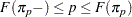 |
where 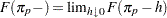 . PROC SEVERITY uses the following practical method of computing . Let
  denote the empirical distribution function (EDF) estimate at a severity value
  . This estimate is computed by PROC SEVERITY and supplied to the name_PARMINIT subroutine. Let
  and
and  denote two consecutive values in the array of values such that
  and
and  . Then, the estimate
  is computed as
 |
where  and
and  .
.
Let  denote the smallest double-precision floating-point number such that
  . This machine precision constant can be obtained by using the CONSTANT function in Base SAS software.
The details of how parameters are initialized for each predefined distribution model are as follows:
- BURR
The parameters are initialized by using the method of moments. The
th raw moment of the Burr distribution is: 
Three moment equations
 (
( ) need to be solved for initializing the three parameters of the distribution. In order to get an approximate closed form solution, the second shape parameter
  is initialized to a value of
  . If
. If  , then simplifying and solving the moment equations yields the following feasible set of initial values:
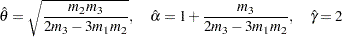
If
 , then the parameters are initialized as follows:
- EXP
The parameters are initialized by using the method of moments. The
th raw moment of the exponential distribution is: 
Solving
 yields the initial value of
  .
. - GAMMA
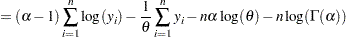
The parameter
 is initialized by using its approximate maximum likelihood (ML) estimate. For a set of iid observations (), drawn from a gamma distribution, the log likelihood,
  , is defined as follows:

Using a shorter notation of
 to denote
  and solving the equation
  yields the following ML estimate of
  :
: 
Substituting this estimate in the expression of
and simplifying gives 
Let
 be defined as follows:
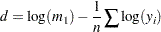
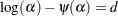
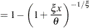
Solving the equation
 yields the following expression in terms of the digamma function,
  :
: 
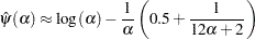
The digamma function can be approximated as follows:
This approximation is within 1.4% of the true value for all the values of
 except when is arbitrarily close to the positive root of the digamma function (which is approximately 1.461632). Even for the values of that are close to the positive root, the absolute error between true and approximate values is still acceptable (
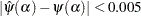 for
for  ). Solving the equation that arises from this approximation yields the following estimate of :
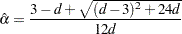
If this approximate ML estimate is infeasible, then the method of moments is used. The
th raw moment of the gamma distribution is: 
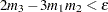
Solving
and  yields the following initial value for :
If
 (almost zero sample variance), then is initialized as follows:
After computing the estimate of
, the estimate of is computed as follows: 
Both the maximum likelihood method and the method of moments arrive at the same relationship between
 and
and  .
. - GPD
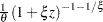
The parameters are initialized by using the method of moments. Notice that for
 , the CDF of the generalized Pareto distribution (GPD) is:

This is equivalent to a Pareto distribution with scale parameter
 and shape parameter
  . Using this relationship, the parameter initialization method used for the PARETO distribution model is used to get the following initial values for the parameters of the GPD distribution model:
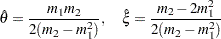
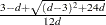
If
(almost zero sample variance) or  , then the parameters are initialized as follows:
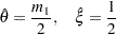
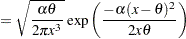
- IGAUSS
The parameters are initialized by using the method of moments. Note that the standard parameterization of the inverse Gaussian distribution (also known as the Wald distribution), in terms of the location parameter
and shape parameter  , is as follows (Klugman, Panjer, and Willmot 1998, p. 583):


For this parameterization, it is known that the mean is
 and the variance is
  , which yields the second raw moment as
 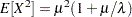 (computed by using
 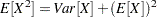 ).
). The predefined IGAUSS distribution model in PROC SEVERITY uses the following alternate parameterization to allow the distribution to have a scale parameter,
: 
The parameters
(scale) and (shape) of this alternate form are related to the parameters and of the preceding form such that  and
and  . Using this relationship, the first and second raw moments of the IGAUSS distribution are:


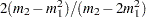
Solving
and yields the following initial values: 
If
(almost zero sample variance), then the parameters are initialized as follows: 
- LOGN
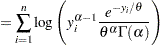
The parameters are initialized by using the method of moments. The
th raw moment of the lognormal distribution is: 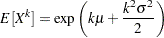
Solving
and yields the following initial values: 
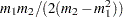
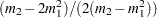
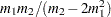
- PARETO
The parameters are initialized by using the method of moments. The
th raw moment of the Pareto distribution is: 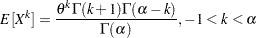
Solving
and yields the following initial values: 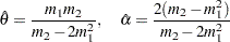
If
(almost zero sample variance) or , then the parameters are initialized as follows: 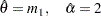
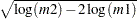
- WEIBULL
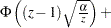
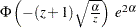
The parameters are initialized by using the percentile matching method. Let
 and
and  denote the estimates of the
  th and
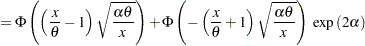
  th percentiles, respectively. Using the formula for the CDF of Weibull distribution, they can be written as
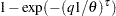

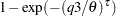

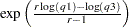
Simplifying and solving these two equations yields the following initial values:
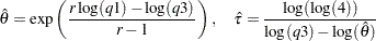
where
 . These initial values agree with those suggested in Klugman, Panjer, and Willmot (1998).
A summary of the initial values of all the parameters for all the predefined distributions is given in Table 22.4. The table also provides the names of the parameters to use in the INIT= option in the DIST statement if you want to provide a different initial value.
Distribution |
Parameter |
Name for INIT option |
Default Initial Value |
|---|---|---|---|
BURR |
|
theta |
|
|
alpha |
|
|
|
gamma |
|
|
EXP |
|
theta |
|
GAMMA |
|
theta |
|
|
alpha |
|
|
GPD |
|
theta |
|
|
xi |
|
|
IGAUSS |
|
theta |
|
|
alpha |
|
|
LOGN |
|
mu |
|
|
sigma |
|
|
PARETO |
|
theta |
|
|
alpha |
|
|
WEIBULL |
|
theta |
|
|
tau |
|
|
Notes: |
|||
|
|||
|
|||
|
|||
|
|||


Note: This procedure is experimental.
Copyright © SAS Institute, Inc. All Rights Reserved.