| The SEVERITY Procedure |
| A Simple Example of Fitting Predefined Distributions |
The simplest way to use PROC SEVERITY is to fit all the predefined distributions to a set of values and let the procedure identify the best fitting distribution.
Consider a lognormal distribution, whose probability density function (PDF)  and cumulative distribution function (CDF)
  are as follows, respectively, where
  denotes the CDF of the standard normal distribution:
 |
The following DATA step statements simulate a sample from a lognormal distribution with population parameters  and
and  , and store the sample in the variable Y of a data set WORK.TEST_SEV1:
 /*------------- Simple Lognormal Example -------------*/
 data test_sev1(keep=y label='Simple Lognormal Sample');
     call streaminit(45678);
     label y='Response Variable';
     Mu = 1.5;
     Sigma = 0.25;
     do n = 1 to 100;
         y = exp(Mu) * rand('LOGNORMAL')**Sigma;
         output;
     end;
 run;
The following statements enable ODS Graphics, fit all the predefined distribution models to the values of Y, and identify the best distribution according to the corrected Akaike’s information criterion (AICC):
 ods graphics on;

 proc severity data=test_sev1;
     model y / crit=aicc;
 run;
The ODS GRAPHICS ON statement enables PROC SEVERITY to generate the default graphics, the PROC SEVERITY statement specifies the input data set, and the MODEL statement specifies the variable to be modeled along with the model selection criterion.
Some of the default output displayed by this step is shown in Figure 22.1 through Figure 22.5. First, information about the input data set is displayed followed by the model selection table, as shown in Figure 22.1. The model selection table displays the convergence status, the value of the selection criterion, and the selection status for each of the candidate models. The Converged column indicates whether the estimation process for a given distribution model has converged, might have converged, or failed. The Selected column indicates whether a given distribution has the best fit for the data according to the selection criterion. For this example, the lognormal distribution model is selected, because it has the lowest value for the selection criterion.
| Input Data Set | |
|---|---|
| Name | WORK.TEST_SEV1 |
| Label | Simple Lognormal Sample |
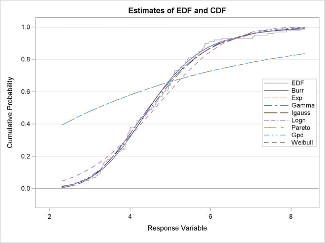
Next, two comparative plots are prepared. These plots enable you to visually verify how the models differ from each other and from the nonparametric estimates. The plot in Figure 22.2 displays the cumulative distribution function (CDF) estimates of all the models and the estimates of the empirical distribution function (EDF). The CDF plot indicates that the Exp (exponential), Pareto, and Gpd (generalized Pareto) distributions are a poor fit as compared to the EDF estimate. The Weibull distribution is also a poor fit, although not as poor as exponential, Pareto, and Gpd. The other four distributions seem to be quite close to each other and to the EDF estimate.
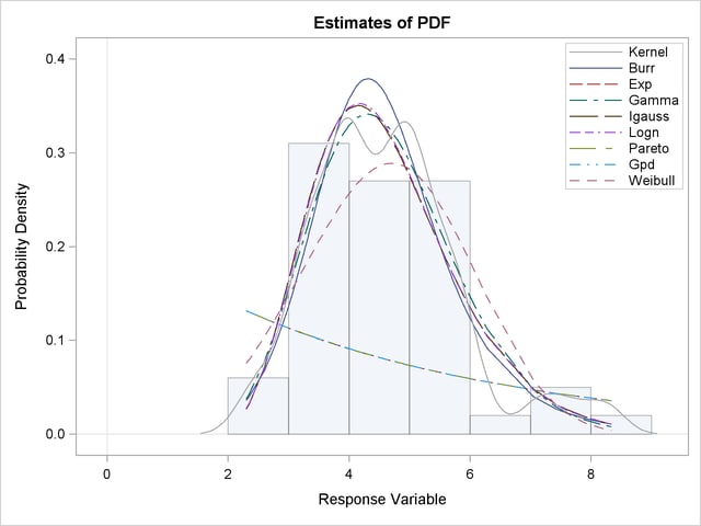
The plot in Figure 22.3 displays the probability density function (PDF) estimates of all the models and the nonparametric kernel and histogram estimates. The PDF plot enables better visual comparison between the Burr, Gamma, Igauss (inverse Gaussian), and Logn (lognormal) models. The Burr and Gamma differ significantly from the Igauss and Logn distributions in the central portion of the range of Y values, while the latter two fit the data almost identically. This provides a visual confirmation of the information in the model selection table of Figure 22.1, which indicates that the AICC values of Igauss and Logn distributions are very close.
The comparative plots are followed by the estimation information for each of the candidate models. The information for the lognormal model, which is the best fitting model, is shown in Figure 22.4. The first table displays a summary of the distribution. The second table displays the convergence status. This is followed by a summary of the optimization process which indicates the technique used, the number of iterations, the number of times the objective function was evaluated, and the log likelihood attained at the end of the optimization. Since the model with lognormal distribution has converged, PROC SEVERITY displays its statistics of fit and parameter estimates. The estimates of Mu=1.49605 and Sigma=0.26243 are quite close to the population parameters of Mu=1.5 and Sigma=0.25 from which the sample was generated. The  -value for each estimate indicates the rejection of the null hypothesis that the estimate is 0, implying that both the estimates are significantly different from 0.
| Distribution Information | |
|---|---|
| Name | Logn |
| Description | Lognormal Distribution |
| Number of Distribution Parameters | 2 |
| Optimization Summary for Logn Distribution | |
|---|---|
| Optimization Technique | Trust Region |
| Number of Iterations | 2 |
| Number of Function Evaluations | 8 |
| Log Likelihood | -157.72104 |
| Fit Statistics for Logn Distribution | |
|---|---|
| -2 Log Likelihood | 315.44208 |
| Akaike's Information Criterion | 319.44208 |
| Corrected Akaike's Information Criterion | 319.56579 |
| Schwarz's Bayesian Information Criterion | 324.65242 |
| Kolmogorov-Smirnov Statistic | 0.50641 |
| Anderson-Darling Statistic | 0.31240 |
| Cramer-von Mises Statistic | 0.04353 |
| Parameter Estimates for Logn Distribution | ||||
|---|---|---|---|---|
| Parameter | Estimate | Standard Error |
t Value | Approx Pr > |t| |
| Mu | 1.49605 | 0.02651 | 56.43 | <.0001 |
| Sigma | 0.26243 | 0.01874 | 14.00 | <.0001 |
The parameter estimates of the Burr distribution are shown in Figure 22.5. These estimates are used in the next example.
Note: This procedure is experimental.
Copyright © SAS Institute, Inc. All Rights Reserved.