Details :: SAS/ETS(R) 9.22 User's Guide

Details

Declining Balance (DB)

Recall that the straight line method assumes a constant depreciation value. Conversely, the declining balance method assumes a constant depreciation rate per year. And like the sum-of-years method, more depreciation tends to occur earlier in the asset’s life.

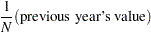
Assume the price of a depreciating asset is $\text{[math]}$ and its salvage value after $\text{[math]}$ years is $\text{[math]}$ . You could assume the asset depreciates by a factor of $\text{[math]}$ (or a rate of $\text{[math]}$ ). This method is known as single declining balance. The annual depreciation is:

$\text{[math]}$

So for our example, the depreciation during the first year is $\text{[math]}$ . Table 53.3 describes how declining balance would depreciate the asset.

Table 53.3 Declining Balance Example
Year	Depreciation	Year-End Value
1	$\text{[math]}$	$\text{[math]}$
2	$\text{[math]}$	$\text{[math]}$
3	$\text{[math]}$	$\text{[math]}$
4	$\text{[math]}$	$\text{[math]}$
5	$\text{[math]}$	$\text{[math]}$

DB Factor

You could also accelerate the depreciation by increasing the factor (and hence the rate) at which depreciation occurs. Other commonly accepted depreciation rates are $\text{[math]}$ (called double declining balance as the depreciation factor becomes $\text{[math]}$ ) and $\text{[math]}$ . Investment Analysis enables you to choose between these three types for declining balance: 2 (with $\text{[math]}$ depreciation), 1.5 (with $\text{[math]}$ ), and 1 (with $\text{[math]}$ ).

Declining Balance and the Salvage Value

The declining balance method assumes that depreciation is faster earlier in an asset’s life; this is what you wanted. But notice the final value is greater than the salvage value. Even if the salvage value were greater than $6,553.60, the final year-end value would not change. The salvage value never enters the calculation, so there is no way for the salvage value to force the depreciation to assume its value. Newnan and Lavelle (1998) describe two ways to adapt the declining balance method to assume the salvage value at the final time. One way is as follows:

Suppose you call the depreciated value after $\text{[math]}$ years $\text{[math]}$ . This sets $\text{[math]}$ and $\text{[math]}$ .

If $\text{[math]}$ according to the usual calculation for $\text{[math]}$ , redefine $\text{[math]}$ to equal $\text{[math]}$ .
If $\text{[math]}$ according to the usual calculation for $\text{[math]}$ for some $\text{[math]}$ (and hence for all subsequent $\text{[math]}$ values), you can redefine all such $\text{[math]}$ to equal $\text{[math]}$ .

This alteration to declining balance forces the depreciated value of the asset after $\text{[math]}$ years to be $\text{[math]}$ and keeps $\text{[math]}$ no less than $\text{[math]}$ .

Conversion to SL

The second (and preferred) way to force declining balance to assume the salvage value is by conversion to straight line. If $\text{[math]}$ , the first way redefines $\text{[math]}$ to equal $\text{[math]}$ ; you can think of this as converting to the straight line method for the last timestep.

If the $\text{[math]}$ value supplied by DB is appreciably larger than $\text{[math]}$ , then the depreciation in the final year would be unrealistically large. An alternate way is to compute the DB and SL step at each timestep and take whichever step gives a larger depreciation (unless DB drops below the salvage value).

After SL assumes a larger depreciation, it continues to be larger over the life of the asset. SL forces the value at the final time to equal the salvage value. As an algorithm, this looks like the following statements:

   V(0) = P;
   for i=1 to N
      if DB step > SL step from (i,V(i))
         take a DB step to make V(i);
      else
         break;
   for j = i to N
      take a SL step to make V(j);

The MACRS, which is discussed in the section that describes the Depreciation Table window, is actually a variation on the declining balance method with conversion to the straight line method.

Top of Page