| The AUTOREG Procedure |
Example 8.6 Estimation of ARCH(2) Process
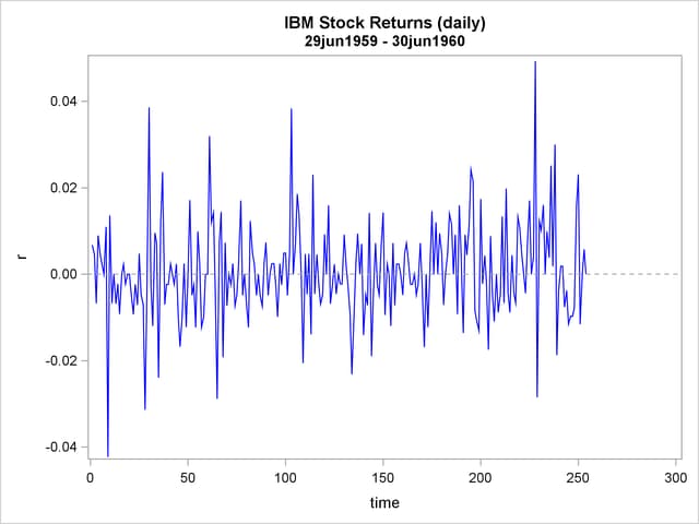
Stock returns show a tendency for small changes to be followed by small changes while large changes are followed by large changes. The plot of daily price changes of IBM common stock (Box and Jenkins; 1976, p. 527) is shown in Output 8.6.1. The time series look serially uncorrelated, but the plot makes us skeptical of their independence.
With the following DATA step, the stock (capital) returns are computed from the closing prices. To forecast the conditional variance, an additional 46 observations with missing values are generated.
title 'IBM Stock Returns (daily)';
title2 '29jun1959 - 30jun1960';

data ibm;
   infile datalines eof=last;
   input x @@;
   r = dif( log( x ) );
   time = _n_-1;
   output;
   return;
last:
   do i = 1 to 46;
      r = .;
      time + 1;
      output;
   end;
   return;
datalines;

   ... more lines ...
 proc sgplot data=ibm;
    series y=r x=time/lineattrs=(color=blue);
          refline 0/ axis = y LINEATTRS = (pattern=ShortDash);
       run;
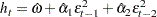
The simple ARCH(2) model is estimated using the AUTOREG procedure. The MODEL statement option GARCH=(Q=2) specifies the ARCH(2) model. The OUTPUT statement with the CEV= option produces the conditional variances V. The conditional variance and its forecast are calculated using parameter estimates:
 |
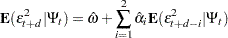 |
where  This model can be estimated as follows:
proc autoreg data=ibm maxit=50;
   model r = / noint garch=(q=2);
   output out=a cev=v;
run;
The parameter estimates for  , and
, and  are 0.00011, 0.04136, and 0.06976, respectively. The normality test indicates that the conditional normal distribution may not fully explain the leptokurtosis in the stock returns (Bollerslev; 1987).
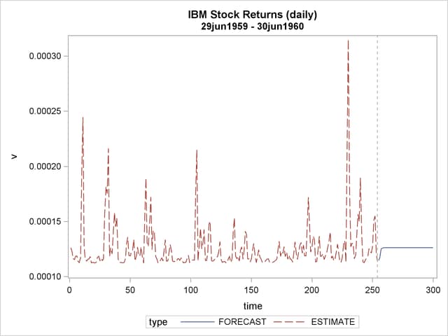
The ARCH model estimates are shown in Output 8.6.2, and conditional variances are also shown in Output 8.6.3. The code that generates Output 8.6.3 is shown below.
data b; set a;
   length type $ 8.;
   if r ^= . then do;
      type = 'ESTIMATE'; output; end;
   else do;
      type = 'FORECAST'; output; end;
run;
proc sgplot data=b;
   series x=time y=v/group=type;
         refline 254/ axis = x LINEATTRS = (pattern=ShortDash);
run;
| Dependent Variable | r |
|---|
| Ordinary Least Squares Estimates | |||
|---|---|---|---|
| SSE | 0.03214307 | DFE | 254 |
| MSE | 0.0001265 | Root MSE | 0.01125 |
| SBC | -1558.802 | AIC | -1558.802 |
| MAE | 0.00814086 | AICC | -1558.802 |
| MAPE | 100.378566 | HQC | -1558.802 |
| Durbin-Watson | 2.1377 | Regress R-Square | 0.0000 |
| Total R-Square | 0.0000 | ||
| NOTE: No intercept term is used. R-squares are redefined. | |||
| GARCH Estimates | |||
|---|---|---|---|
| SSE | 0.03214307 | Observations | 254 |
| MSE | 0.0001265 | Uncond Var | 0.00012632 |
| Log Likelihood | 781.017441 | Total R-Square | 0.0000 |
| SBC | -1545.4229 | AIC | -1556.0349 |
| MAE | 0.00805675 | AICC | -1555.9389 |
| MAPE | 100 | HQC | -1551.7658 |
| Normality Test | 105.8587 | ||
| Pr > ChiSq | <.0001 | ||
| NOTE: No intercept term is used. R-squares are redefined. | |||
Copyright © SAS Institute, Inc. All Rights Reserved.