Previous Page

|

Next Page

The AUTOREG Procedure

Example 8.1 Analysis of Real Output Series

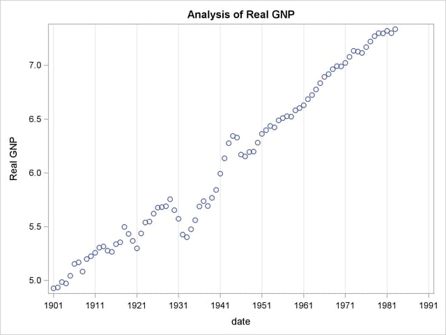
In this example, the annual real output series is analyzed over the period 1901 to 1983 (Balke and Gordon; 1986, pp. 581–583). With the following DATA step, the original data are transformed using the natural logarithm, and the differenced series DY is created for further analysis. The log of real output is plotted in Output 8.1.1.

title 'Analysis of Real GNP';
data gnp;
   date = intnx( 'year', '01jan1901'd, _n_-1 );
   format date year4.;
   input x @@;
   y  = log(x);
   dy = dif(y);
   t  = _n_;
   label y  = 'Real GNP'
         dy = 'First Difference of Y'
         t  = 'Time Trend';
datalines;

   ... more lines ...   

proc sgplot data=gnp noautolegend;
   scatter x=date y=y;
   xaxis grid values=('01jan1901'd '01jan1911'd '01jan1921'd '01jan1931'd
             '01jan1941'd '01jan1951'd '01jan1961'd '01jan1971'd
             '01jan1981'd '01jan1991'd); 
run;   

Output 8.1.1 Real Output Series: 1901 – 1983

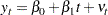
The (linear) trend-stationary process is estimated using the following form:

where

The preceding trend-stationary model assumes that uncertainty over future horizons is bounded since the error term, , has a finite variance. The maximum likelihood AR estimates from the statements that follow are shown in Output 8.1.2:

proc autoreg data=gnp;
   model y = t / nlag=2 method=ml;
run;

Output 8.1.2 Estimating the Linear Trend Model

Analysis of Real GNP

The AUTOREG Procedure

Maximum Likelihood Estimates
SSE	0.23954331	DFE	79
MSE	0.00303	Root MSE	0.05507
SBC	-230.39355	AIC	-240.06891
MAE	0.04016596	AICC	-239.55609
MAPE	0.69458594	HQC	-236.18189
Durbin-Watson	1.9935	Regress R-Square	0.8645
		Total R-Square	0.9947

Parameter Estimates
Variable	DF	Estimate	Standard Error	t Value	Approx Pr > |t|	Variable Label
Intercept	1	4.8206	0.0661	72.88	<.0001
t	1	0.0302	0.001346	22.45	<.0001	Time Trend
AR1	1	-1.2041	0.1040	-11.58	<.0001
AR2	1	0.3748	0.1039	3.61	0.0005

Autoregressive parameters assumed given
Variable	DF	Estimate	Standard Error	t Value	Approx Pr > |t|	Variable Label
Intercept	1	4.8206	0.0661	72.88	<.0001
t	1	0.0302	0.001346	22.45	<.0001	Time Trend

Nelson and Plosser (1982) failed to reject the hypothesis that macroeconomic time series are nonstationary and have no tendency to return to a trend line. In this context, the simple random walk process can be used as an alternative process:

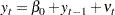where and . In general, the difference-stationary process is written as

where is the lag operator. You can observe that the class of a difference-stationary process should have at least one unit root in the AR polynomial .

The Dickey-Fuller procedure is used to test the null hypothesis that the series has a unit root in the AR polynomial. Consider the following equation for the augmented Dickey-Fuller test:

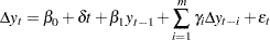where . The test statistic is the usual t ratio for the parameter estimate , but the does not follow a t distribution.

The following code performs the augmented Dickey-Fuller test with and we are interesting in the test results in the linear time trend case since the previous plot reveals there is a linear trend.

proc autoreg data = gnp;
   model y = / stationarity =(adf =3); 
run;

The augmented Dickey-Fuller test indicates that the output series may have a difference-stationary process. The statistic Tau with linear time trend has a value of and its p-value is . The statistic Rho has a p-value of which also indicates the null of unit root is accepted at the 5% level. (See Output 8.1.3.)

The AR(1) model for the differenced series DY is estimated using the maximum likelihood method for the period 1902 to 1983. The difference-stationary process is written

The estimated value of is and that of is 0.0293. All estimated values are statistically significant. The PROC step follows:

proc autoreg data=gnp;
   model dy = / nlag=1 method=ml;
run;

The printed output produced by the PROC step is shown in Output 8.1.4.

Copyright © SAS Institute, Inc. All Rights Reserved.