PROC AUTOREG: Heteroscedasticity and GARCH Models

The AUTOREG Procedure

Heteroscedasticity and GARCH Models

There are several approaches to dealing with heteroscedasticity. If the error variance at different times is known, weighted regression is a good method. If, as is usually the case, the error variance is unknown and must be estimated from the data, you can model the changing error variance.

The generalized autoregressive conditional heteroscedasticity (GARCH) model is one approach to modeling time series with heteroscedastic errors. The GARCH regression model with autoregressive errors is

$\text{[math]}$

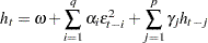This model combines the mth-order autoregressive error model with the GARCH $\text{[math]}$ variance model. It is denoted as the AR $\text{[math]}$ -GARCH $\text{[math]}$ regression model.

The tests for the presence of ARCH effects (namely, Q and LM tests, tests from Lee and King (1993) and tests from Wong and Li (1995)) can help determine the order of the ARCH model appropriate for the data. For example, the Lagrange multiplier (LM) tests shown in Figure 8.11 are significant $\text{[math]}$ through order 12, which indicates that a very high-order ARCH model is needed to model the heteroscedasticity.

The basic ARCH $\text{[math]}$ model $\text{[math]}$ is a short memory process in that only the most recent q squared residuals are used to estimate the changing variance. The GARCH model $\text{[math]}$ allows long memory processes, which use all the past squared residuals to estimate the current variance. The LM tests in Figure 8.11 suggest the use of the GARCH model $\text{[math]}$ instead of the ARCH model.

The GARCH $\text{[math]}$ model is specified with the GARCH=(P= $\text{[math]}$ , Q= $\text{[math]}$ ) option in the MODEL statement. The basic ARCH $\text{[math]}$ model is the same as the GARCH $\text{[math]}$ model and is specified with the GARCH=(Q= $\text{[math]}$ ) option.

The following statements fit an AR(2)-GARCH $\text{[math]}$ model for the Y series that is regressed on TIME. The GARCH=(P=1,Q=1) option specifies the GARCH $\text{[math]}$ conditional variance model. The NLAG=2 option specifies the AR(2) error process. Only the maximum likelihood method is supported for GARCH models; therefore, the METHOD= option is not needed. The CEV= option in the OUTPUT statement stores the estimated conditional error variance at each time period in the variable VHAT in an output data set named OUT. The data set is the same as in the section Testing for Heteroscedasticity.

data c;
   ul=0; ull=0;
   do time = -10 to 120;
      s = 1 + (time >= 60 & time < 90);
      u = + 1.3 * ul - .5 * ull + s*rannor(12346);
      y = 10 + .5 * time + u;
      if time > 0 then output;
      ull = ul; ul = u;
      end;
run;
title 'AR(2)-GARCH(1,1) model for the Y series regressed on TIME';
proc autoreg data=c;
   model y = time / nlag=2 garch=(q=1,p=1) maxit=50;
   output out=out cev=vhat;
run;

The results for the GARCH model are shown in Figure 8.13. (The preliminary estimates are not shown.)

Figure 8.13 AR(2)-GARCH $\text{[math]}$ Model

AR(2)-GARCH(1,1) model for the Y series regressed on TIME

The AUTOREG Procedure

GARCH Estimates
SSE	218.861036	Observations	120
MSE	1.82384	Uncond Var	1.6299733
Log Likelihood	-187.44013	Total R-Square	0.9941
SBC	408.392693	AIC	388.88025
MAE	0.97051406	AICC	389.88025
MAPE	2.75945337	HQC	396.804343
		Normality Test	0.0838
		Pr > ChiSq	0.9590

Parameter Estimates
Variable	DF	Estimate	Standard Error	t Value	Approx Pr > \|t\|
Intercept	1	8.9301	0.7456	11.98	<.0001
time	1	0.5075	0.0111	45.90	<.0001
AR1	1	-1.2301	0.1111	-11.07	<.0001
AR2	1	0.5023	0.1090	4.61	<.0001
ARCH0	1	0.0850	0.0780	1.09	0.2758
ARCH1	1	0.2103	0.0873	2.41	0.0159
GARCH1	1	0.7375	0.0989	7.46	<.0001

The normality test is not significant (p = 0.959), which is consistent with the hypothesis that the residuals from the GARCH model, $\text{[math]}$ , are normally distributed. The parameter estimates table includes rows for the GARCH parameters. ARCH0 represents the estimate for the parameter $\text{[math]}$ , ARCH1 represents $\text{[math]}$ , and GARCH1 represents $\text{[math]}$ .

The following statements transform the estimated conditional error variance series VHAT to the estimated standard deviation series SHAT. Then, they plot SHAT together with the true standard deviation S used to generate the simulated data.

data out;
   set out;
   shat = sqrt( vhat );
run;

title 'Predicted and Actual Standard Deviations';
proc sgplot data=out noautolegend;
   scatter x=time y=s; 
   series x=time y=shat/ lineattrs=(color=black); 
run;

The plot is shown in Figure 8.14.

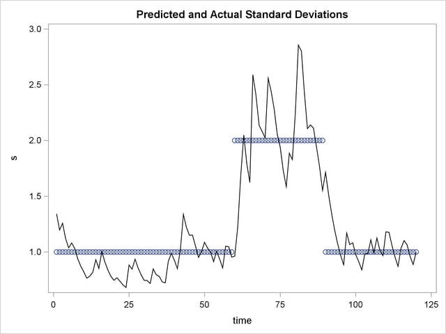
Figure 8.14 Estimated and Actual Error Standard Deviation Series

In this example note that the form of heteroscedasticity used in generating the simulated series Y does not fit the GARCH model. The GARCH model assumes conditional heteroscedasticity, with homoscedastic unconditional error variance. That is, the GARCH model assumes that the changes in variance are a function of the realizations of preceding errors and that these changes represent temporary and random departures from a constant unconditional variance. The data-generating process used to simulate series Y, contrary to the GARCH model, has exogenous unconditional heteroscedasticity that is independent of past errors.

Nonetheless, as shown in Figure 8.14, the GARCH model does a reasonably good job of approximating the error variance in this example, and some improvement in the efficiency of the estimator of the regression parameters can be expected.

The GARCH model might perform better in cases where theory suggests that the data-generating process produces true autoregressive conditional heteroscedasticity. This is the case in some economic theories of asset returns, and GARCH-type models are often used for analysis of financial market data.

GARCH Models

The AUTOREG procedure supports several variations of GARCH models.

Using the TYPE= option along with the GARCH= option enables you to control the constraints placed on the estimated GARCH parameters. You can specify unconstrained, nonnegativity-constrained (default), stationarity-constrained, or integration-constrained models. The integration constraint produces the integrated GARCH (IGARCH) model.

You can also use the TYPE= option to specify the exponential form of the GARCH model, called the EGARCH model, or other types of GARCH models, namely the quadratic GARCH (QGARCH), threshold GARCH (TGARCH), and power GARCH (PGARCH) models. The MEAN= option along with the GARCH= option specifies the GARCH-in-mean (GARCH-M) model.

The following statements illustrate the use of the TYPE= option to fit an AR(2)-EGARCH $\text{[math]}$ model to the series Y. (Output is not shown.)

/*-- AR(2)-EGARCH(1,1) model --*/
proc autoreg data=a;
   model y = time / nlag=2 garch=(p=1,q=1,type=exp);
run;

See the section GARCH Models for details.

Top of Page