SAS Products
SAS Risk Dimensions - Optimizing Portfolios
Overview of Optimizing Portfolios
Setting Up a Working Environment
- Create the Optimization Program
- Use Market, Instrument, and Base Weight Data
- Create a Portfolio File
- Create a Report of the Portfolio Optimization Process
- Update the Portfolio Optimization Program
- Overview of the Example
- Create the Risk Environment
- Optimize the Portfolio
- Run the Portfolio Optimization for a Given Risk Level
Creating an Efficient Frontier and Calculating the Market Portfolio
- Overview of the Example
- Create the Efficient Frontier for the Portfolio
- Calculate the Market Portfolio
- Run the Portfolio Optimization with the Efficient Frontier
Overview
To optimize your portfolio, you need to find the optimal amounts of various assets to hold, given a set of restrictions. You need to consider factors such as risk tolerance, industry or sector exposure, and so on. You have a choice not only of which financial instruments to hold in your portfolio, but also of the proportion of each instrument in the portfolio. You can build any number of portfolios, and each possible portfolio has its own risk-return characteristics.
SAS Risk Dimensions provides a range of options for evaluating and optimizing portfolios. You can optimize in order to maximize return or to minimize one of many risk measures.
In this example, you will complete the following tasks:
- set up a working environment for portfolio optimization
- perform portfolio optimization in order to find the portfolio that maximizes return for a set risk indicator level
- subject that optimized portfolio to additional linear constraints
- create an efficient frontier
This example uses the following fictitious stock ticker symbols:
- XBBA: a telecommunications company
- XBBB: a bank
- XBBC: a technology company
- XBBD: a regional utility
- XBBE: an oil company
- XBBF: an automobile maker
- XBBG: a software company
- XBBH: a global energy company
- XBBI: a retail chain
- XBBJ: a supermarket chain
For simplicity, only capital gains are used to represent returns in this example. Dividends are ignored.
The ZIP file for this example contains the following data set and programs:
| Program | Description |
| OptDat.sas7bdat | Contains historical prices of the 10 fictitious stocks. |
| MktInstWeightData.sas | Creates input data sets. See Use Market, Instrument, and Base Weight Data for the complete description of these data sets. |
| WeightMacro.sas | Defines the SAS macro that creates a weighted portfolio. This instrument data set contains the instruments based on portfolio value, current market prices, and a weighting scheme. |
| OptReportMacro.sas | Defines the SAS macro that creates the final report for the optimization process. |
| RiskSetupA.sas | Initializes the SAS Risk Dimensions environment and registers the required variables. |
| CalcOptPortfolio.sas | Analyzes and optimizes the initial portfolio. |
| CalcOptPortfolio2.sas | Creates linear constraints and optimizes the portfolio subject to those constraints. |
| EfFrontier.sas | Creates an efficient frontier data set and fits a model to that data by using SAS Risk Dimensions. |
| CalcMktPortfolio.sas | Finds the market portfolio by using the efficient frontier. |
Storing Your Data
Before you proceed, make sure that the RD_Examples directory is accessible to SAS Risk Dimensions. See Creating a Directory to Store Your Data for instructions.
Setting Up a Working Environment
Create the Optimization Program
To create the optimization program:
- In the SAS Enhanced Editor window, enter the following statements:
%let loc = C:\users\sasdemo\RD_Examples\;
libname rdexamp clear;
libname rdexamp "&loc";
%let pValue = 5000000;
The SAS macro variable &LOC now contains the path to the example directory C:\users\sasdemo\RD_Examples.The macro variable &PVALUE contains the dollar value of the portfolio, which is set to $5,000,000.
The library RDExamp is created, which points to the example directory.
- Save the contents of the SAS Enhanced Editor window into a file named Optimization.sas in the directory. As you proceed through this example, you update this optimization program.
- Extract optdat.sas7bdat from the ZIP file into the example directory. This data set contains historical prices of the 10 fictitious stocks. The environment that you have created and the subsequent analyses use this data set to estimate a covariance matrix, which SAS Risk Dimensions needs for simulation of stock prices.
Use Market, Instrument, and Base Weight Data
Extract MktInstWeightData.sas from the ZIP file and copy it to C:\users\sasdemo\RD_Examples.
Here is the code from that file:
/* Create the market data set */
data RDExamp.Mkt_Data;
	     informat Date date7.;
    	 format Date date7.;
         input Date P_XBBA P_XBBB P_XBBC P_XBBD P_XBBE P_XBBF P_XBBG P_XBBH
                    P_XBBI P_XBBJ;
datalines;
	30May14 39.9 34.01 23.06 18.48 88.76 17.1 28.32 42.76 57.74 13.34
;

/* Create the instrument data set without number of shares. */
data RDExamp.Inst_Data_wo;
  	input InstType $ InstID $ Company $ ;
			Mkt_P = ("P_" || InstID);
datalines;
  Stock XBBA Telco
  Stock XBBB Bank
  Stock XBBC Tech
  Stock XBBD Utility
  Stock XBBE Oil
  Stock XBBF Auto
  Stock XBBG Software
  Stock XBBH Energy
  Stock XBBI Retail
  Stock XBBJ Food
;

/* Create a Base Weighting Scheme with equal weights. */
data RDExamp.wght;
	    input Company $ wgt;
datalines;
    Telco 0.1
    Bank 0.1
    Tech 0.1
    Utility 0.1
    Oil 0.1
    Auto 0.1
    Software 0.1
    Energy 0.1
    Retail 0.1
    Food 0.1
;
This program creates three input data sets:
- Mkt_Data, which contains the current market value of the instruments.
- Inst_Data_wo, which contains instrument definitions without the holdings of each instrument.
- Wght, which contains the weighting scheme for the portfolio. You assume that each stock is equally weighted, but you could assign different weights if you wanted. This weight data set is used by the %CREATINSTSET macro to appropriately weight the instrument data set Inst_Data_wo.
You include this program in Optimization.sas later in the example.
Create a Portfolio File
Extract WeightMacro.sas from the ZIP file and save it in C:\users\sasdemo\RD_Examples.
Here is the code from that file:
	%macro CreateInstSet(inDir, inMktPrc, inWgt, inInstSet,
                            outSet, value=1000000);
	/* Begin PROC SQL.   */
	proc sql noprint;

	/* Create a temporary output table for the portfolio file. */
	   create table temp_out
	   (   InstType        Char(8),
  		 InstID          Char(8),
	   	 P_ID            Char(10),
	   	 Holding         num,
		    Company         Char(15)
   	);

/* Create a temporary table for rearranging MKT prices. */
   create table temp_mktprc as
	      select *
		      from &inDir..&inMktPrc;

/* Create the MKT price table. */
	   create table new_mktprc
	      (   P_ID            Char(10),
			    Price           num
	      );

/* Drop the date field from the temp MKT price table. */
	   alter table temp_mktprc
	   drop Date;

/* Populate the temporary out table with the values from the holding */
/* field to the portfolio value times the security weight.           */
	   insert into temp_out (InstType, InstID,
				                   P_ID, Holding,
				                   Company)
	   select a.InstType, a.InstID,
			    a.Mkt_P,(b.wgt*&value),
			    a.Company
	      from &inDir..&inInstSet as a,
		        &inDir..&inWgt as b
	      where a.company = b.company;

/* Count the number of securities in the output table. */
/* Store the value in a SAS macro table.               */
   select count(P_ID)
	      into :n_mkt
    	from temp_out;

/* Read the values of P_ID into a series of macro variables. */
  	select P_ID
	      into :ID1 - :ID%left(&n_mkt)
    	from temp_out;

/* Loop over the # of IDs.    */
%do i=1 %to &n_mkt;

/* Create a pointer to the current P_ID.  */
	%let tmpa = &&ID&i;

/* Select MKT price for the current P_ID.  */
/* Store in a macro.                       */
   select &tmpa
	      into :prc
    	from temp_mktprc;

/* Insert current P_ID and price into new MKT price table. */
  	insert into new_mktprc
	      values( "&tmpa", &prc );

%end ;

/* Update the temporary out table dividing holding by MKT price. */
	update temp_out as a
	set Holding = Holding / (
	select Price
	   from new_mktprc as b
  	where a.P_ID = b.P_ID);

/* Round the holding value.   */
	update temp_out
	   set Holding = round(Holding);

/* End PROC SQL.              */
quit;

/* Use a DATA step to update the output data set. */
data &inDir..&outSet;
	   set temp_out;
		drop P_ID;
;

%mend CreateInstSet;
This program defines a macro that completes the following steps when it runs:
- creates temporary output and market price tables for ease of manipulation.
- creates a new market price table in an easy-to-use format.
- populates the temporary output table with the data from the instrument definition set. Sets the holding value to the dollar amount to be invested.
- loops through the temporary market price table and stores the price data in the new market price table.
- updates the temporary holding values for the output table. Divides the current value (the dollar amount) by the market price to calculate the number of shares to hold. Rounds the number of shares to the nearest integer.
- uses a SAS DATA step to set the output data set to the temporary output data set.
You include this program in Optimization.sas later in the example.
Create a Report of the Portfolio Optimization Process
Extract OptReportMacro.sas from the ZIP file and save it in C:\users\sasdemo\RD_Examples.
Here is the code from that file:
%macro WriteReport(inDir, env_name, Proj, es);

/* Libref to project output. */
	%let inpath=%sysfunc(pathname(&inDir,L));
	%if %index(&inpath,\) %then %let sep=\; %else %let sep=/;
	libname projdir "&inpath.&sep.&env_name.&sep.&Proj";

proc sql;

/* Create a new data set containing the optimal weights. */
	create table &inDir..OptWgt as
	   select Company,
	          OptWeight as wgt "Optimal Weight"
		   from projdir.optvalue
		   where Company <> "+";

quit;

/*Use the Portfolio Generation macro to create the optimal portfolio.*/
%CreateInstSet(&inDir,Mkt_Data,OptWgt,Inst_Data_wo,Opt_Inst_Data,value=&pValue);

proc sql;

/* Create a new table to contain the relevant information */
/* for the report.                                        */
	   create table &indir..OptReport
	      (Company      Char(15)    label="Company*Name",
			 Holding      num        label="Optimal*Holding",
			 opt_wgt      num        label="Optimal*Weight",
		    old_wgt      num        label="Original*Weight",
		    old_holding  num        label="Original*Holding",
		    amt_sell     num        label="Amount*to Sell"
		    );

/* Populate the table with the information.   */
   insert into &inDir..OptReport (Company,
                                  Holding,
                                  opt_wgt, old_wgt,
                                  old_holding, amt_sell)
    select a.Company,
				  a.Holding,
				  b.wgt,
				  c.wgt,
				  d.Holding,
				  (d.Holding - a.Holding)
    from  &inDir..Opt_Inst_Data as a,
				   &inDir..OptWgt        as b,
				   &inDir..wght          as c,
				   &inDir..Inst_Data     as d
	where (a.Company = b.Company) AND
				(b.Company = c.Company) AND
				(c.Company = d.Company);
quit;

title "Project: &Proj";
title2 "Constraint: Expected Shortfall = &ES";

/* Use PROC REPORT to generate the formatted report. */
proc report data = &inDir..OptReport box nowindows split="*";
	   Column Company old_wgt opt_wgt old_holding Holding
				  to_sell to_buy;

		define   old_wgt             / display format=6.4;
	    define   opt_wgt             / display format=6.4;
		define   old_holding         / display;
		define   Holding             / display;
		define   to_sell             / computed "Amount*to Sell"
				                         format=6.0;
		define   to_buy              / computed "Amount*to Buy"
				                         format=6.0;

		compute to_sell;
				  to_sell = old_holding - Holding;
				  if to_sell < 0 then to_sell = 0;
		endcomp;
		compute to_buy;
				  to_buy = Holding - old_holding;
				  if to_buy < 0 then to_buy = 0;
		endcomp;
run;

title;

proc report data = projdir.optsum
	   box nowindows split="*";

		column   AnalysisName BaseDate _date_
				   objectivename constraintname
				   constraintRHS CurObjective
				   OptObjective;
		define   analysisname      / display "Name*of*Analysis";
		define   basedate          / display "Base*Case*Date";
		define   _date_            / display "Valuation*Date";
		define   objectivename     / display "Objective";
		define   constraintname    / display "Constraint";
		define   constraintRHS     / display "Constraint*=";
		define   CurObjective      / display "Original*Expected*Return"
				                       format=6.4;
		define   OptObjective      / display "Optimal*Expected*Return"
				                       format=6.4;
run;

libname projdir clear;
%mend WriteReport;
This program defines a macro that completes the following steps when it runs:
- uses PROC SQL to create the optimal weight data set from the SAS Risk Dimensions output files
- uses the CreateInstSet macro with the optimal weight data set to create a new optimal instrument data set
- uses PROC SQL to populate a data set for reporting that contains the relevant information
- uses PROC REPORT to create a report of the information that is stored in the data set that was created by PROC SQL
- uses PROC REPORT to summarize the overall changes in the characteristics of the optimized portfolio
You include this program in Optimization.sas in the next section.
Update the Portfolio Optimization Program
Update the optimization program, Optimization.sas:
- Open Optimization.sas in the SAS Enhanced Editor.
- Update the contents of the file with the following code:
%let loc = C:\users\sasdemo\RD_Examples\;
	libname rdexamp clear;
	libname rdexamp "&loc";
	%let pValue = 5000000;

	%include "&loc.MktInstWeightData.sas";
	%include "&loc.WeightMacro.sas";
	%include "&loc.OptReportMacro.sas";

/* Create the instrument portfolio set */
	%CreateInstSet(RDExamp,Mkt_Data,wght,Inst_Data_wo,Inst_Data,value=&pValue);
This code includes the programs that you extracted previously. It runs the CreateInstSet macro with the following arguments:- RDExamp: the SAS Risk Dimensions library
- Mkt_Data: table of current market prices
- Wght: table of weights for the portfolio
- Inst_Data_wo: instrument definition data set
- Inst_Data: output data set, which is the weighted portfolio
- Value: value of the portfolio
- Save the program as Optimization.sas in the C:\users\sasdemo\RD_Examples directory.
Optimizing a Portfolio for a Given Risk Level
Overview of the Example
Now you can optimize the return of a portfolio of stocks for a specified level of risk. Specifically, you can find an optimal weighting scheme for your portfolio so that it maximizes the expected return while holding the risk level constant.
First, you analyze the risk of your initial portfolio. From that analysis, you find the expected shortfall as a percentage of the total portfolio value, which is used as the constraint for the optimization. Expected shortfall is the expected value of loss, conditional on loss being above value at risk (VaR). For this example, short positions are not allowed.
Create the Risk Environment
Extract RiskSetupA.sas from the ZIP file and copy it to C:\users\sasdemo\RD_Examples.
Here is the code from that file:
/* RiskSetupA.sas creates the risk environment. */
	   proc risk;
/* Create a new environment. */
	      environment new = RDExamp.optimex;
/* Create instrument variables. */
	      declare instvars = (
			   	  Company  char 15 class label = "Issuing company");
/* Create risk factor variables.
    Use the form
           P_<ticker> num var
                      label "<company> share price"
                      refmap = (compref = "<company>") */
		   declare riskfactors = (
           P_XBBA num var
                  label = "Telco share price"
                  refmap = (compref = "Telco"),
           P_XBBB num var
                  label = "Bank share price"
                  refmap = (compref = "Bank"),
           P_XBBC num var
                  label = "Tech share price"
                  refmap = (compref = "Tech"),
           P_XBBD num var
                  label = "Utility share price"
                  refmap = (compref = "Utility"),
           P_XBBE num var
                  label = "Oil share price"
                  refmap = (compref = "Oil"),
           P_XBBF num var
                  label = "Auto share price"
                  refmap = (compref = "Auto"),
           P_XBBG num var
                  label = "Software share price"
                  refmap = (compref = "Software"),
           P_XBBH num var
                  label = "Energy share price"
                  refmap = (compref = "Energy"),
           P_XBBI num var
                  label = "Retail share price"
                  refmap = (compref = "Retail"),
           P_XBBJ num var
                  label = "Food share price"
                  refmap = (compref = "Food"));
/* Create a reference variable. */
	      declare reference = (compref num var
	                           label = "Company" );
/* Create a cross-classification. */
	      crossclass cc1 (Company);
       environment save;
run;

/* Create a pricing method program. */
proc compile outlib = RDexamp.optimex
	                environment = RDexamp.optimex
	                package = Stock_Price;
/* Pricing function for stocks. */
	      function stock_price(price)
         kind = pricing
	         label = "Simple stock pricing function";
	         return(price);
      endsub;
/* Create the stock pricing method. */
	      method Stock_Price desc = "Simple stock pricing method"
	                         kind = Price;
	         _value_ = compref.company;
      endmethod;
 	run;

/* The COVAR macro is used to create a covariance matrix, which   */
/* is needed for the covariance simulation.                       */
%covar("&loc", OptDat, "&loc", Cov_Data, Cov_Mat, RDExamp.optimex ,1,,,,);

/* Create the stock instrument and register the instrument data. */
proc risk;
	      environment open = RDExamp.optimex;
/* Create a stock instrument. */
	      instrument Stock
	         label = "Stock"
		      variables = (Holding, Company)
	         methods = (price Stock_Price);
/* Register the instrument data. */
	      instdata Stock_Data
		      file = RDExamp.Inst_Data
		      format = simple
		      variables = (InstType InstID Holding Company);
/* Create a portfolio list for stocks. */
      sources Stock_List Stock_Data ;
/* Create a portfolio file for stocks. */
	      read sources = Stock_List out = Stock_File;
/* Register the market data. */
	       marketdata Mkt_Data
	          file = RDExamp.Mkt_Data
	          type = current;
/* Register the covariance matrix. */
	      marketdata Cov_Mat
	         file = RDExamp.Cov_Data
		      type = covariance
		      interval = weekday;
		   environment save;
run;

/* Create the weight bounds. */
data RDExamp.stockbound;
      input Company $ InstID $ lb ub;
datalines;
     Telco XBBA . 1.0
     Bank XBBB . 1.0
     Tech XBBC . 1.0
     Utility XBBD . 1.0
     Oil XBBE . 1.0
     Auto XBBF . 1.0
     Software XBBG . 1.0
     Energy XBBH . 1.0
     Retail XBBI . 1.0
     Food XBBJ . 1.0
;
This program completes the following steps:
- creates the SAS Risk Dimensions environment
- creates the instrument, risk factor, and cross-classification variables
- creates a basic pricing method
- creates the covariance matrix from the historical data that is required for the covariance simulation
- registers the instrument data and creates the portfolio
- registers the current market data and the covariance matrix
- creates a data set to constrain the portfolio weights
Linear constraints are addressed in Optimizing a Portfolio with Linear Constraints. For more information, see the OPTIMIZATION statement in SAS Risk Dimensions and SAS High-Performance Risk: Procedures Guide.
Optimize the Portfolio
Extract CalcOptPortfolio.sas from the ZIP file and copy it to C:\users\sasdemo\RD_Examples.
Here is the code from that file:
/* Analyze the initial portfolio.  Optimize the weighting scheme
	for the same level of risk. */
proc risk;
   environment open = RDExamp.optimex;
/* Set analysis options. */
	      setoptions optsummary;
/* Create a simulation analysis using the      */
/* covariance matrix created in RiskSetupA.sas */
	      simulation Stock_Sim
	         interval = weekday
	         method = covariance
	         seed = 12345
		      ndraw = 1500
		      data = Cov_Mat
	         horizon = (1);
/* Create the analysis project Stock_Proj. */
      project Stock_Proj
	         data = (Mkt_Data)
	         portfolio = Stock_File
	         analysis = (Stock_Sim)
	         numeraire = USD
	         rundate = "30May14"d
	         crossclass = cc1
		      out = Initial_Stock_Results;
/* Run the analysis project. */
		   runproject Stock_Proj
	         options = (outall);
		   environment save;
run;

/* Create library to Initial_Stock_Results. */
%macro createlib;
		   %let inpath=%sysfunc(pathname(RDExamp,L));
			%if %index(&inpath,\) %then %let sep=\; %else %let sep=/;
			libname stockres "&loc.&sep.optimex&sep.Initial_Stock_Results";
%mend;

%createlib;

/* Use SQL to store ES as a macro variable in a macro. */
proc sql noprint;
	      select ES / MtM
		      into :ESPct
		      from stockres.simstat
	         where Company = "+";
quit;

proc risk;
	   environment open = RDExamp.optimex;
/* Set analysis options. */
	      setoptions optsummary;
/* Create an optimization analysis. */
	      optimization Stock_Optimization
	         simulation = Stock_Sim
	         horizon = (1)
		      objective = return
		      subjectto = (es = (&ESPct))
		      bounds = RDExamp.stockbound;
/* Create the analysis project Stock_Opt_Proj. */
	      project Stock_Opt_Proj
		      data = (Mkt_Data)
	         portfolio = Stock_File
		      analysis = (Stock_Optimization)
	         numeraire = USD
		      rundate = "30May14"d
		      crossclass = cc1
	         out = Optimal_Stock_Results;
/* Run the analysis project. */
				runproject Stock_Opt_Proj
				   options = (outall);
				environment save;
run;

libname stockres clear;
This program completes the following steps:
- creates a covariance simulation with a horizon of one weekday.
- creates and runs a project that is based on the covariance simulation.
- uses a PROC SQL statement to calculate and store the expected shortfall (ES) as a percentage of mark-to-market in a SAS macro variable.
- creates an optimization analysis based on the covariance simulation, maximizing return. The analysis is subject to the ES equaling the initial ES and the portfolio weighting bounds.
- creates and runs a project by using the optimization analysis
Run the Portfolio Optimization for a Given Risk Level
Update the optimization program, Optimization.sas:
- Open Optimization.sas in the SAS Enhanced Editor.
- Update the contents of the file with the following code:
%let loc = C:\users\sasdemo\RD_Examples\;
libname rdexamp clear;
	libname rdexamp "&loc";
%let pValue = 5000000;

%include "&loc.MktInstWeightData.sas";
%include "&loc.WeightMacro.sas";
%include "&loc.OptReportMacro.sas";

/* Create the instrument portfolio set */
%CreateInstSet(RDExamp,Mkt_Data,wght,Inst_Data_wo,Inst_Data,value=&pValue);

/* Use ODS to output the reports in html */
	   ods listing close;
	   ods html body = "&loc.optimization_body.htm"
			        contents="&loc.TOC.htm"
			        frame="&loc.optimization.htm";

%include "&loc.RiskSetupA.sas";
%include "&loc.CalcOptPortfolio.sas";
%WriteReport(RDExamp, optimex, Optimal_Stock_Results,&ESPct);

ods html close;
- Save the program as Optimization.sas in the C:\users\sasdemo\RD_Examples directory.
- Execute Optimization.sas by clicking
 .
. - Check the SAS Log window for errors. If there are errors, correct them and rerun the program.
The following report is generated.
Portfolio Optimization Report Optimization for a Given Risk Level
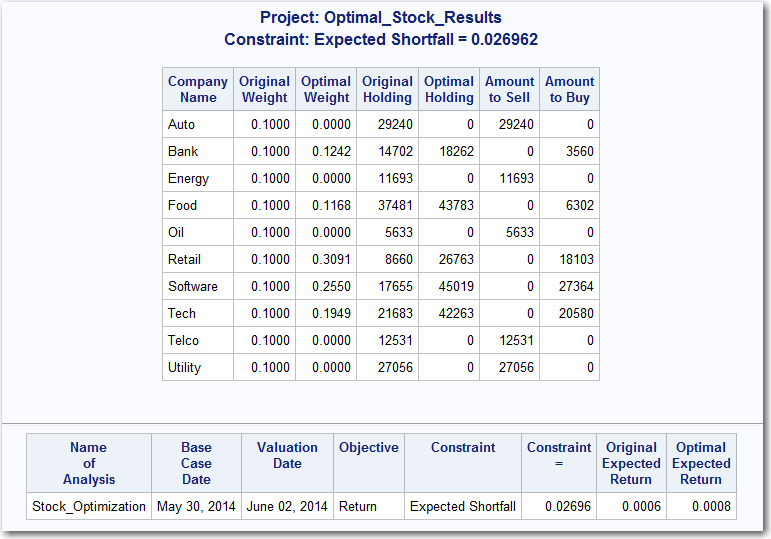
The first table summarizes the original and optimal portfolios. The columns of the table and their contents are as follows:
| Table Column | Contents |
| Company Name | Name of the company |
| Original Weight | Initial portfolio weights for each company |
| Optimal Weight | Weights for the optimized portfolio |
| Original Holding | Number of shares owned in the initial portfolio |
| Optimal Holding | Number of shares to hold in the optimal portfolio |
| Amount to Sell | Number of shares of each company to sell in order to attain the optimal portfolio |
| Amount to Buy | Number of shares of each company to buy in order to attain the optimal portfolio |
The second table summarizes the optimization procedure. The columns of the table and their contents are as follows:
| Table Column | Contents |
| Name of Analysis | SAS Risk Dimensions name of the optimization analysis |
| Base Case Date | Date of the optimization |
| Valuation Date | Date on which the portfolio is valued |
| Objective | Optimization objective (maximize return or minimize risk) |
| Constraint | Constraint used in the optimization |
| Constraint = | Value of the constraint |
| Original Expected Return | Expected return over the holding period (one day in this case) for the initial portfolio |
| Optimal Expected Return | Expected return over the holding period for the optimized portfolio |
Optimizing a Portfolio with Linear Constraints
Overview of the Example
The OPTIMIZATION statement in PROC RISK supports additional linear constraints in the optimization problem. For example, you could allow only a specified percentage of the total value in a given sector, or maybe a specified amount in a combination of stocks. The BOUNDS and LINCON options in the OPTIMIZATION statement support these constraints.
The BOUNDS option specifies the weight bounds for individual cross-classification cells. The only cross-classification variable is the company. The StockBound data set that was created in RiskSetupA.sas is an example of this type of constraint.
The LINCON option specifies linear relationships across the cross-classification cells. This relationship is illustrated in the following section.
For more information about constraints, see the OPTIMIZATION statement in SAS Risk Dimensions and SAS High-Performance Risk: Procedures Guide.
Create Linear Constraints
Extract CalcOptPortfolio2.sas from the ZIP file and copy it to C:\users\sasdemo\RD_Examples.
Here is the code from that file:
/* CalcOptPortfolio2.sas creates the linear constraints and optimizes */
	/* the portfolio subject to those constraints.                   */

data RDExamp.stocklin;
	      input CName $ CType $ Company $ CCoef;
datalines;
	cons1 le .    0.20
	cons1 .  Auto 1
	cons2 le .    0.30
	cons2 .  Tech 1
	cons2 .  Software 1
	cons3 le .    0.30
	cons3 .  Utility 1
	cons3 .  Energy 1
	cons3 .  Oil 1
;

proc risk;
	  environment open = RDExamp.optimex;
/* Set analysis options. */
	      setoptions optsummary;
/* Create an optimization analysis. */
	      optimization Stock_Optimization2
	         simulation = Stock_Sim
	         horizon = (1)
	         objective = return
	         subjectto = (es = (&ESPct))
	         bounds = RDExamp.stockbound
	         lincon = RDExamp.stocklin;
/* Create the analysis project Stock_Opt. */
      project Stock_Opt_Proj2
         data = (Mkt_Data)
	         portfolio = Stock_File
	         analysis = (Stock_Optimization2)
	         numeraire = USD
	         rundate = "30May14"d
	         crossclass = cc1
	         out = Optimal_Stock_Results2;
/* Run the analysis project. */
      runproject Stock_Opt_Proj2
	         options = (outall);
      environment save;
run;
This program creates the linear constraint file and optimizes the portfolio by using the following constraints:
- No more than 20% of the portfolio value is allowed in automotive stocks: weight_XBBF = 20%
- No more than 30% of the portfolio value is allowed in technology and software stocks: weight_XBBC + weight_XBBG = 30%
- No more than 30% of the portfolio value is allowed in utility, energy, and oil stocks: weight_XBBD + weight_XBBH + weight_XBBG = 30%
Run the Optimization with Linear Constraints
Update the optimization program, Optimization.sas:
- Open Optimization.sas in the SAS Enhanced Editor.
- Update the contents of the file with the following code:
%let loc = C:\users\sasdemo\RD_Examples\;
libname rdexamp clear;
libname rdexamp "&loc";
%let pValue = 5000000;

%include "&loc.MktInstWeightData.sas";
%include "&loc.WeightMacro.sas";
%include "&loc.OptReportMacro.sas";

/* Create the instrument portfolio set */
%CreateInstSet(RDExamp,Mkt_Data,wght,Inst_Data_wo,Inst_Data,value=&pValue);

/* Use ODS to output the reports in html */
	   ods listing close;
	   ods html body = "&loc.optimization_body.htm"
	      contents="&loc.TOC.htm"
	      frame="&loc.optimization.htm";

%include "&loc.RiskSetupA.sas";
%include "&loc.CalcOptPortfolio.sas";
%WriteReport(RDExamp, optimex, Optimal_Stock_Results,&ESPct);

%include "&loc.CalcOptPortfolio2.sas";
%WriteReport(RDExamp, optimex, Optimal_Stock_Results2,&ESPct);

ods html close;
- Save the program as Optimization.sas in the C:\users\sasdemo\RD_Examples directory.
- Execute Optimization.sas by clicking .
- Check the SAS Log window for errors. If there are errors, correct them and rerun the program.
The following report is generated and appended to the previously generated output.
Portfolio Optimization Report Optimization with Linear Constraints
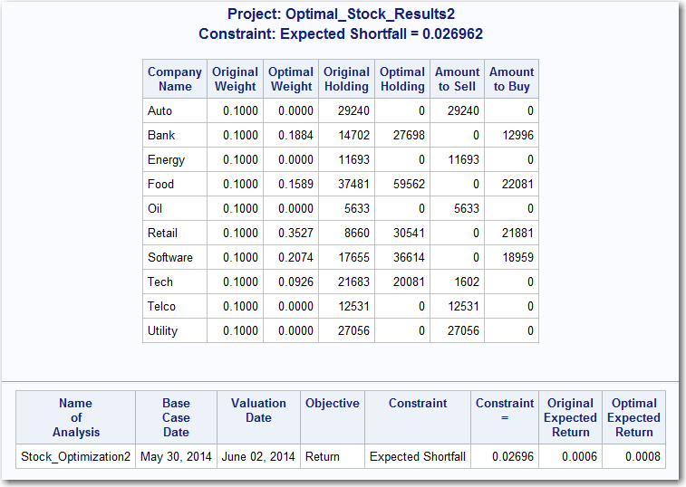
Note: The optimal portfolio weights changed because the linear constraints were added to the optimization problem. All of the linear constraints are binding.
- Automotive stock constraint : weight_XBBF = 20%
- Technology stock constraint: weight_XBBC + weight_XBBG = 29.57% + 0.43% = 30%
- Energy and oil stock constraint: weight_XBBD + weight_XBBH + weight_XBBE = 20.49% + 9.51% = 30%
Notice that the optimal expected return is unchanged from the unconstrained optimal portfolio.
Creating an Efficient Frontier and Calculating the Market Portfolio
Overview of the Example
So far, you have optimized a portfolio for a single expected shortfall value. Optimizing over a range of expected shortfalls yields an optimal risk-return curve. This curve is called the efficient frontier.
The capital market line is defined as the line tangent to the efficient frontier whose intercept is the risk-free rate of return. The point of tangency characterizes the market portfolio.
Create the Efficient Frontier for the Portfolio
Extract EfFrontier.sas from the ZIP file and copy it to C:\users\sasdemo\RD_Examples.
Here is the code from that file:
/*  EfFrontier.sas finds and fits an efficient frontier
	for the portfolio.   */
proc risk;
			environment open = RDExamp.optimex;
/* Set analysis options. */
      setoptions optsummary;
/* Create an optimization analysis. */
	      optimization Eff_Frontier
	      simulation = Stock_Sim
	         horizon = (1)
		       objective = return
		       subjectto = (es = (0.023 to 0.038 by 0.001))
	         bounds = RDExamp.stockbound
	         lincon = RDExamp.stocklin;
/* Create the analysis project Stock_Opt. */
	      project Stock2_Proj
	         data = (Mkt_Data)
	         portfolio = Stock_File
	         analysis = (Eff_Frontier)
	         numeraire = USD
	         rundate = "30May14"d
	         crossclass = cc1
         out = EF_Results;
/* Run the analysis project. */
       runproject Stock2_Proj
	         options = (outall);
       environment save;
run;

/* Create library to Efficient Frontier results. */
%macro createlib;
	   %let inpath=%sysfunc(pathname(RDExamp,L));
	   %if %index(&inpath,\) %then %let sep=\; %else %let sep=/;
	   libname effres "&loc.&sep.optimex&sep.ef_results";
%mend;

%createlib;

/* Create a quadratic data set from the risk/return profile  */
/* of the efficient frontier.                                */
data risk_return;
	      set effres.optsum
	      (keep = OptObjective OptConstraint);
			  OO2 = OptObjective**2;
;

/* Output the parameter estimates from PROC REG. */
	   ods output ParameterEstimates = RDExamp.estimates
	      (drop= Model DF Dependent StdErr tValue Probt);

/* OLS regression of the efficient frontier. */
	   proc reg data = risk_return;
	      model OptConstraint = OO2 OptObjective;
	   quit;

	   libname effres clear;
This program completes the following steps:
- creates an optimization analysis with 17 expected shortfall constraints (that is, from ES = 0.023...0.038 by 0.001).
- creates and runs a project based on the optimization analysis.
- creates a SAS data set from the output of SAS Risk Dimensions.
- uses PROC REG to perform an ordinary least squares (OLS) regression on the data set that is created from the SAS Risk Dimensions output.
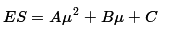
The efficient frontier is modeled as the quadratic equation
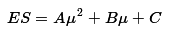
where µ is the optimal return, and A, B, and C are estimated parameters.
Calculate the Market Portfolio
Extract CalcMktPortfolio.sas from the ZIP file and copy it to C:\users\sasdemo\RD_Examples.
Here is the code from that file:
/* CalcMktPortfolio.sas uses the fitted variables of the efficient frontier to
	find the market portfolio. */

/* Risk-Free Daily RoR. */
%let r_free = 0.000111;

proc sql noprint;
/* Get the fitted intercept. */
      select estimate
	         into :c
	         from RDExamp.estimates
	         where variable = "Intercept";

/* Get the fitted quadratic parameter. */
	      select estimate
	         into :a
	         from RDExamp.estimates
	         where variable = "OO2";

	* Get the fitted linear parameter. */
	      select estimate
         into :b
	         from RDExamp.estimates
	         where variable = "OptObjective";

/* Use the risk-free RoR and the parameters to calculate  */
/* the RoR of the market portfolio.                       */
	         insert into RDExamp.estimates
	         set variable = "Mkt RoR",
		          estimate = (2*&a*&r_free +
			                   sqrt((4*(&a**2)*&r_free**2 +
			                   4*&a*(&r_free*&b + &c) )))
			                   / (2*&a);

/* Get the mkt portfolio RoR. */
	         select estimate
			      into :u
			      from RDExamp.estimates
			      where variable = "Mkt RoR";

/* Calculate the ES of the mkt portfolio. */
			   insert into RDExamp.estimates
			      set variable = "Mkt ES",
			          estimate = &a*&u**2 + &b*&u + &c;

/* Get the ES of the mkt portfolio. */
			   select estimate
			      into :r_mkt
			      from RDExamp.estimates
			      where variable = "Mkt ES";
quit;

/* Use PROC RISK to create the mkt portfolio weights. */
proc risk;
	   environment open = RDExamp.optimex;
/* Set analysis options. */
		 setoptions optsummary;
/* Create an optimization analysis. */
       optimization Stock_Optimization3
          simulation = Stock_Sim
	          horizon = (1)
		       objective = return
	          subjectto = (es = (&r_mkt))
	          bounds = RDExamp.stockbound
	          lincon = RDExamp.stocklin;
/* Create the analysis project Mkt_Portfolio. */
	       project Mkt_Portfolio
			          data = (Mkt_Data)
			          portfolio = Stock_File
			          analysis = (Stock_Optimization3)
			          numeraire = USD
			          rundate = "30May14"d
			          crossclass = cc1
			          out = Mkt_Portfolio;
/* Run the analysis project. */
			 runproject Mkt_Portfolio
			    options = (outall);
			 environment save;
 run;
This program completes the following steps:
- sets a SAS macro variable to the 90-day U.S. Treasury daily return for May 30, 2014 (.04/360 = .000111). In this example, that value is the risk-free rate of return, rf.
- uses PROC SQL to calculate the risk and return of the market portfolio.
- uses SAS Risk Dimensions to calculate the asset weights of the market portfolio.
Run the Portfolio Optimization with the Efficient Frontier
Update the optimization program, Optimization.sas:
- Open Optimization.sas in the SAS Enhanced Editor.
- Update the contents of the file with the following code:
%let loc = C:\users\sasdemo\RD_Examples\;
	libname rdexamp clear;
	libname rdexamp "&loc";
	%let pValue = 5000000;

%include "&loc.MktInstWeightData.sas";
%include "&loc.WeightMacro.sas";
%include "&loc.OptReportMacro.sas";

/* Create the instrument portfolio set */
%CreateInstSet(RDExamp,Mkt_Data,wght,Inst_Data_wo,Inst_Data,value=&pValue);

/* Use ODS to output the reports in html */
   ods listing close;
		ods html body = "&loc.optimization_body.htm"
	       contents="&loc.TOC.htm"
			 frame="&loc.optimization.htm";

%include "&loc.RiskSetupA.sas";
%include "&loc.CalcOptPortfolio.sas";
%WriteReport(RDExamp, optimex, Optimal_Stock_Results,&ESPct);

%include "&loc.CalcOptPortfolio2.sas";
%WriteReport(RDExamp, optimex, Optimal_Stock_Results2,&ESPct);

%include "&loc.EfFrontier.sas";
%include "&loc.CalcMktPortfolio.sas";
%WriteReport(RDExamp, optimex, Mkt_Portfolio, &r_mkt);

ods html close;
- Save the program as Optimization.sas in the C:\users\sasdemo\RD_Examples directory.
- Execute Optimization.sas by clicking .
- Check the SAS Log window for errors. If there are errors, correct them and rerun the program.
The following reports are generated and appended to the previous output. This report shows the output from PROC REG.
PROC REG Output Efficient Frontier Estimation
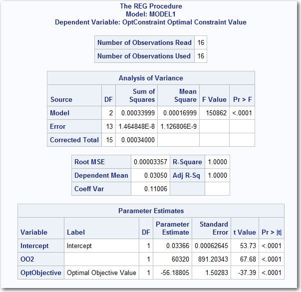
The expected shortfall is modeled as a quadratic equation of the optimal return.
PROC REG estimates the parameters as follows:
- A = 60320
- B = 56.18805
- C = 0.03366
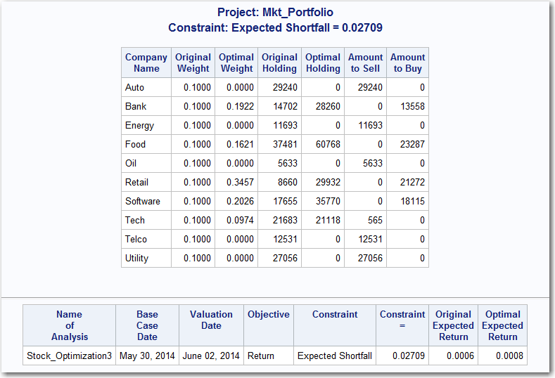
The following report shows the share weights, risk level, and expected return of the market portfolio.
Portfolio Optimization Report Market Portfolio