SAS Products
SAS Risk Dimensions - Using Copula Aggregation with the AGGREGATION Procedure
Define the Marginal Distribution Data Set
Provide Input Data for Copulas and Marginal Distributions
Overview
Aggregation might be necessary when portions of a company's risk are calculated independently from one another. For example, market risk and credit risk might be calculated separately, but a joint risk measure would be useful. Aggregation allows the merging of these two measurements while accounting for correlations between them.
A copula is a function that combines marginal distributions of variables into a specific multivariate distribution. Using copulas can help you perform large-scale multivariate simulation from separate models, each of which can be fitted using different, even non-normal, distributional specifications. Copula-based aggregation allows for a mix of univariate distributions at the lowest or leaf level of a hierarchy.
The AGGREGATION procedure supports a hierarchical approach to copula aggregation, which does not require a specification of relationships between sub-portfolios. Instead, you specify the joint dependence between the aggregated sub-portfolios in successive steps of aggregation. This allows the use of different copulas for each aggregation step. Hence, you can combine a variety of copula dependence structures and properties. This hierarchical copula approach can be considered a copula specification dimension reduction tool. The mixed copula approach efficiently reduces the risk aggregation to n subset decisions on the best fit copula.
Objective
This example involves a company that aggregates its risk on multiple levels. At the top of the hierarchy is the company level, which is comprised of business units, which in turn are made up of regional operations. Within each region, activity is further broken down by strategy. The following figure shows this organization.
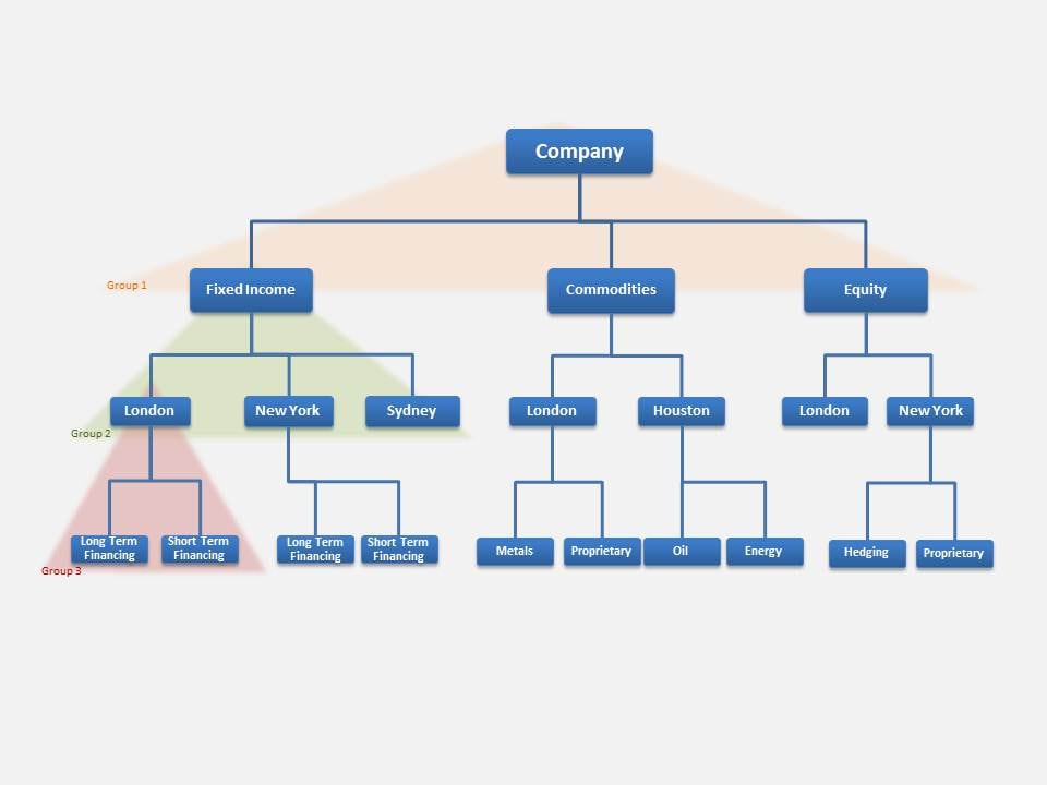
It is important to clearly understand the hierarchical structure of a project when using the AGGREGATION procedure. The figure above depicts distinct levels of aggregation and their components. When you use the AGGREGATION procedure, you identify these clusters of aggregation and components as "groups." Groups 1, 2, and 3 of the project are highlighted in the figure.
In Group 3, the components are Long Term Financing and Short Term Financing and the aggregation is to the London region.
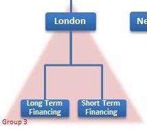
For each group, you need to specify how to aggregate the components. Starting with Group 3, you need to identify the copula for aggregation and assign marginal distributions to the components.
Assume that Long Term Financing profit/loss has a normal distribution with mean zero and standard deviation of 500. Assume that Short Term Financing profit/loss has a student's t-distribution with three degrees of freedom. The Group 3 copula is a Clayton copula with theta set to 0.3.
Moving up to Group 2, identify the copula for aggregation and the marginal distribution for the Sydney region because it has not yet been defined. After this continue the process for all nodes of the tree.
After you have defined copulas and distributions for groups, run the AGGREGATION procedure to simulate marginal components and do copula aggregation. You can request simulation values and statistics to see the risk measures for the components and aggregations.
The AGGREGATION procedure does not require the environment set up and project steps required for the RISK procedure.
Set Up Your Environment
Assign the library RDExamp. Use the directory C:\users\sasdemo\RD_Examples. In this code, you use the SAS Macro Language Facility to create the macro variable test_lib. You assign the value of RDExamp, which is the library name that was assigned in the previous libname statement, to the variable test_lib.
%let test_lib = RDExamp;
Define the Configuration Data
The configuration data set specifies the structure of the aggregation and defines the copulas and marginal distributions. In this example, there are three levels of aggregation. First you aggregate strategies into regions, then regions into business units, and finally business units into the firmwide level. The configuration data set has columns for the cross classifications as well as for copula, marginal distribution, output variable, group name, and reference name.
|
data &test_lib..config; length unit $32 region $32 strategy $32 copula $32 marginal $32 var $32 group $32 REFNAME $32; input unit $ region $ strategy $ copula $ marginal $ var $ group $ refname; datalines; |
|
FixedIncome + + copula1 nosrc PL group1 FITotal Commodities + + copula1 nosrc PL group1 CommodTotal Equity + + copula1 nosrc PL group1 EQTotal FixedIncome London + copula2 nosrc PL group2 FILondon FixedIncome NewYork + copula2 nosrc PL group2 FINewYork FixedIncome Sydney + copula2 marg1 PL group2 FISydney FixedIncome London LongTermFinancing copula3 marg2 PL group3 FILondonLTF FixedIncome London ShortTermFinancing copula3 marg3 PL group3 FILondonSTF FixedIncome NewYork LongTermFinancing copula4 marg4 PL group4 FINewYorkLTF FixedIncome NewYork ShortTermFinancing copula4 marg5 PL group4 FINewYorkSTF Commodities London + copula5 nosrc PL group5 CommodLondon Commodities Houston + copula5 nosrc PL group5 CommodHouston Commodities London Metals copula6 marg6 PL group6 CommodLondonMet Commodities London Proprietary copula6 marg7 PL group6 CommodLondonProp Commodities Houston Oil copula7 marg8 PL group7 CommodHoustonOil Commodities Houston Energy copula7 marg9 PL group7 CommodHoustonEnergy Equity London + copula8 marg10 PL group8 EQLondon Equity NewYork + copula8 nosrc PL group8 EQNewYork Equity NewYork Hedging copula9 marg11 PL group9 EQNewYorkHDG Equity NewYork Proprietary copula9 marg12 PL group9 EQNewYorkProp |
| ; |
Define the Copula Data Set
The copula data set defines the copulas for aggregation. The names of the copulas must match the names specified in your configuration data set.
|
data RDExamp.copula; length name $32 parameter $32 CValue $32; input name $ parameter $ CValue $ NValue; datalines; |
|
copula1 type t . copula1 cov RDExamp.UnitCorr . copula1 df . 10 copula2 type t . copula2 cov RDExamp.FIRegionCorr . copula2 df . 25 copula3 type clayton . copula3 theta . 0.70 copula4 type clayton . copula4 theta . 0.60 copula5 type frank . copula5 theta . 1 copula6 type clayton . copula6 theta . 65 copula7 type clayton . copula7 theta . 4 copula8 type normal . copula8 cov RDExamp.EQRegionCorr . copula9 type Frank . copula9 theta . .5 |
| ; |
Define the Marginal Distribution Data Set
The marginal distribution data set describes the marginal distributions specified in the configuration data set.
|
data RDExamp.marginal; length name $32 parameter $32 CValue $32; input name $ parameter $ CValue $ NValue ; datalines; |
|
marg1 type NORMAL . marg1 args . 2 marg1 parm . 1000 marg1 parm . 500000 marg2 type NORMAL . marg2 args . 2 marg2 parm . 20000 marg2 parm . 450000 marg3 type NORMAL . marg3 args . 2 marg3 parm . 1500 marg3 parm . 200000 marg4 type NORMAL . marg4 args . 2 marg4 parm . 350 marg4 parm . 175000 marg5 type NORMAL . marg5 args . 2 marg5 parm . 2150 marg5 parm . 150000 marg6 type NORMAL . marg6 args . 2 marg6 parm . 53000 marg6 parm . 1000 marg7 type NORMAL . marg7 args . 2 marg7 parm . 800 marg7 parm . 2000 marg8 type NORMAL . marg8 args . 2 marg8 parm . 10 marg8 parm . 15000 marg9 type NORMAL . marg9 args . 2 marg9 parm . 650 marg9 parm . 1800 marg10 type NORMAL . marg10 args . 2 marg10 parm . 100 marg10 parm . 14000 marg11 type NORMAL . marg11 args . 2 marg11 parm . 2300 marg11 parm . 1000 marg12 type EMPIRICAL . marg12 source RDExamp.EQNewYorkProp . |
| ; |
Provide Input Data for Copulas and Marginal Distributions
Some copulas and marginal distributions require input data. You can provide empirical distribution data or correlation matrices. The following code defines several correlation data sets and one empirical distribution data set.
|
data RDExamp.UnitCorr; length _name_ $12; input _name_ $ _type_ $ FITotal CommodTotal EQTotal; datalines; |
|
FITotal corr 1 .25 .35 CommodTotal corr .25 1 .3 EQTotal corr .35 .3 1 |
| ; |
|
data RDExamp.FIRegionCorr; length _name_ $12; input _name_ $ _type_ $ FILondon FINewYork FISydney; datalines; |
|
FILondon corr 1 .45 .40 FINewYork corr .45 1 .50 FISydney corr .40 .50 1 |
| ; |
|
data RDExamp.EQRegionCorr; length _name_ $12; input _name_ $ _type_ $ EQLondon EQNewYork; datalines; |
|
EQLondon corr 1 .35 EQNewYork corr .35 1 |
| ; |
data RDExamp.EQNewYorkProp;
format _date_ date9.;
length refname $32.;
input refname $ _date_ date9. replication PL;
datalines;
|
EQNewYorkProp 25MAY2011 1 956.72 EQNewYorkProp 29MAY2011 2 438.57 EQNewYorkProp 30MAY2011 3 564.76 EQNewYorkProp 31MAY2011 4 456.11 EQNewYorkProp 01JUN2011 5 229.23 EQNewYorkProp 04JUN2011 6 270.67 EQNewYorkProp 05JUN2011 7 1158.99 EQNewYorkProp 06JUN2011 8 408.93 EQNewYorkProp 07JUN2011 9 1207.44 EQNewYorkProp 08JUN2011 10 1535.40 EQNewYorkProp 11JUN2011 11 800.34 EQNewYorkProp 12JUN2011 12 1574.01 EQNewYorkProp 13JUN2011 13 689.35 EQNewYorkProp 14JUN2011 14 208.58 EQNewYorkProp 15JUN2011 15 -1307.27 EQNewYorkProp 18JUN2011 16 766.56 EQNewYorkProp 19JUN2011 17 231.87 EQNewYorkProp 20JUN2011 18 -277.57 EQNewYorkProp 21JUN2011 19 639.86 EQNewYorkProp 22JUN2011 20 926.39 |
| ; |
Run the AGGREGATION procedure
Now that you have defined all of the input data, run the AGGREGATION procedure. The following code registers the data and runs the procedure. It specifies output data sets for the simulated values and simulation statistics.
vars =(pl comptype=pl)
ccv =(unit region strategy)
config_data = RDExamp.config
copula_spec= RDExamp.copula
marginal_spec= RDExamp.marginal
alpha=0.05
seed = 1234
ndraws = 100000
out_simdata = RDExamp.simdata
out_statdata = RDExamp.statdata
;
runaggr;
run;
View Results
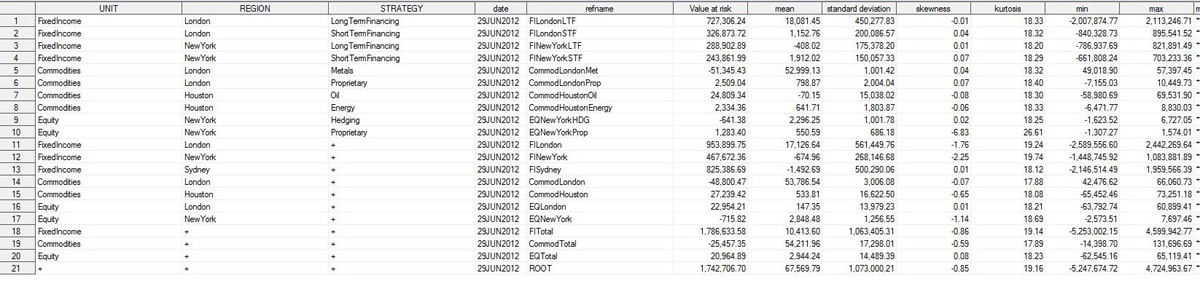
You specified output data sets for the simulated values and simulation statistics. The following figure shows the simulated values data set.
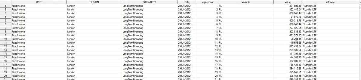
Here is the simulation statistics data set.