If your model involves a function of a predictor variable, such as log(X), various statistics for assessing the effect of a predictor in the model assess the effect of the transformed variable rather than of the original, untransformed variable. For example, in an ordinary regression model including Z=log(X) as a predictor, the parameter estimate for Z is the estimated slope on log(X), not on X itself. While a good fit to the response might require the use of log(X) as a predictor rather than X, you might still be interested in estimating the slope on X. As another example, if Z is a predictor in a logistic model, the estimated odds ratio for Z assesses the effect of Z on the odds, not the effect of X, but you still might want to know what the odds ratio is for X.

A similar situation is when the predictor is involved in a spline effect and assessment of the original variable, rather than of the spline effect, is desired. This situation is discussed and illustrated in SAS Note 70221. SAS Note 67024 addresses the assessment of a continuous predictor more generally.

This question essentially asks how the model prediction changes when X, not Z, is increased by some amount. For example, in an ordinary regression model, the slope is the change in the predicted response mean when you increase the predictor by one unit. So, one way to assess the slope on Z is to evaluate the model at z=log(x) and z+1=log(x)+1 and take their difference to see the change from increasing Z by one unit. But to assess the slope on X, you want to evaluate the model at log(x) and at log(x+1). More generally, to assess the effect of changing X by u units, compare model evaluations at log(x) and at log(x+u).^Note

In some cases, if you write out the model before and after the increase, the difference simplifies to a constant or an expression that you can evaluate. With the simple regression model, E(Y) = α+βX, the change in the estimated mean response for a one unit increase in X is [a+b(x+1)] - [a+bx] = b, which is the estimated slope parameter for X. But for the model E(Y) = δ+γZ = δ+γlog(X), the difference for a one unit increase in X is [δ+γlog(x+1)] - [δ+γlog(x)] = γ[log(x+1)-log(x))] = γlog((x+1)/x), which now depends on X. This makes sense because the model is linear in Z so the slope on Z is the same everywhere, but it is nonlinear in X so the slope changes depending on the X value where the increase is made.

Fortunately, it is not necessary to do this evaluation and simplification process. After fitting your model, you can use the NLEST macro to compute the desired assessment statistic (difference, ratio, or other) using the model expression with and without the desired amount of change. It can then provide the estimated assessment statistic even if the ultimate function of the model parameters is nonlinear. For details about using the NLEST macro and for additional examples, see its documentation in SAS Note 58775.

This approach can be used for any generalized linear model using any link function and can compute the assessment statistic of interest for any transformation of the predictor (log, square root, or other). While simple, one-predictor models are shown in the examples below, it can be used for more complex model specifications. It is important to properly write each model expression in the macro matching the specification used in modeling procedure. Any procedure fitting a generalized linear model (GLIMMIX, GENMOD, LOGISTIC, and others) can be used to fit the model as long as it either supports the STORE statement or can save its parameter estimates and covariance matrix tables.

Simple Regression Model with Log Transformed Predictor

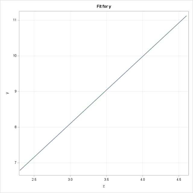
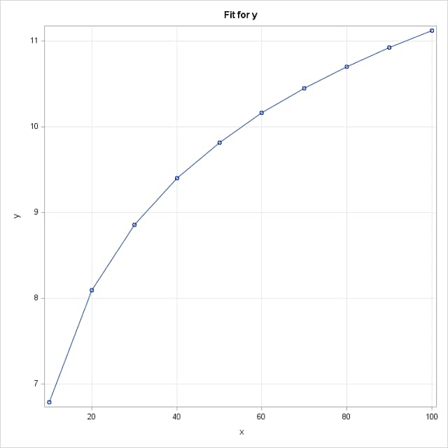
Consider, as discussed above, the simple regression model, E(Y) = δ+γlog(X). The following DATA step simulates data from this model with δ=2 and γ=2. PROC GENMOD then fits and saves the model. A plot of the fitted model on Z is provided by the EFFECTPLOT statement and on X by using PROC SGPLOT to plot the predicted values saved with the OUTPUT statement.

As shown above, the estimated slope at any value of X is γ[log(x+1)-log(x))] = γlog((x+1)/x). Because this is a constant multiplier on the Z parameter, γ, the estimated slope at X=20 can be obtained with the ESTIMATE statement by either specifying the coefficient on Z as log(21/20)=0.04879 or using the SYSFUNC macro function to evaluate log(21/20) or by evaluating [log(x+1)-log(x))] using SYSFUNC and SYSEVALF macro functions, all as shown below:

   data a;
      do x=10 to 100 by 10;
      do r=1 to 5;
         z=log(x);
         y=2 + 2*z + rannor(482);
         output;
      end; end;
      run;
   proc genmod data=a;
      model y=z;
      output out=out p=pred;
      effectplot / noclm;
      estimate '@20' z %sysevalf( %sysfunc(log(21)) - %sysfunc(log(20)) );
      estimate '@20' z %sysfunc(log(21/20));
      estimate '@20' z 0.04879;
      store mod;
      run;
   proc sgplot data=out noautolegend;
      scatter y=pred x=x; 
      series y=pred x=x; 
      xaxis grid; yaxis grid label="y"; 
      title "Fit for y";
      run;

The results from fitting the model to the simulated data approximate the true model parameters. The equivalent specifications of the ESTIMATE statement provide a slope estimate at X=20 of 0.092. Notice that the fitted model is linear on Z=log(X) as is obvious from the true model specification, but is nonlinear on X:

The ESTIMATE statement cannot be used for other generalized linear models that involve link functions other than the identity link used in this example. The more general solution is to use the NLEST macro. As suggested above, you can write out the model before and after the desired increase and use the macro to evaluate the resulting expression. There is no need to simplify the expression unless desired, and it might be a safer to avoid errors when simplifying. The unsimplified code is also likely to be more understandable if viewed later or by another person.

To use the macro, specify the name of the saved model from the STORE statement in instore=, and then specify the difference expression comparing the model before and after increase in f=. Note that the parameters of the fitted model are represented in the f= expression with the names b_p1, b_p2, and so on, in the order shown in the modeling procedure results. Adding a label and title is optional.

The following macro calls estimate the slope using a one unit increase at each of X=20 and X=80:

   %nlest(instore=mod,
          f=(b_p1+b_p2*log(20+1))-(b_p1+b_p2*log(20)),
          title=Slope, label=X=20)
          
   %nlest(instore=mod,
          f=(b_p1+b_p2*log(80+1))-(b_p1+b_p2*log(80)),
          title=Slope, label=X=80)

Compare these estimated slopes to the above plot of the fitted model on X. So, while the slope on Z=log(X) is 2 (actual, but estimated as 1.88) at any value of X since it is linear in Z, the slope on X changes depending on where the increase is made and is estimated to be 0.092 at X=20 and 0.023 at X=80. Note the agreement with the ESTIMATE statement results above for X=20:

A Logistic Model with Log-Transformed Predictor

Consider a similar logistic model with Z=log(X) as a predictor where want to estimate the odds ratio of X as well as Z. In this case, and for any generalized linear model not using the identity link, the ESTIMATE statement cannot be used as it was in the previous example. The NLEST macro can be used to obtain odds ratio estimates for X. But as above with the slope, the odds ratio is not constant in X as it is in Z, so you must specify values of X at which you want odds ratio estimates.

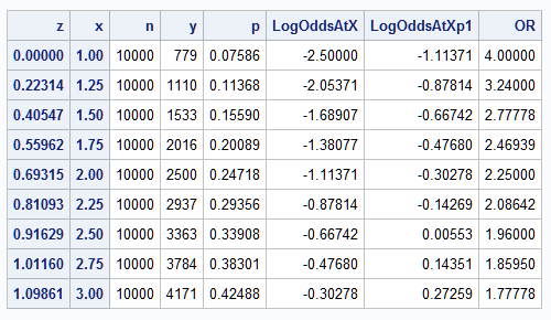
The following statements simulate data from the logistic model logit(Pr(Y)) = -2.5 + 2*log(X). For each value of X between 1 and 3, the true event probability is computed and used to generate a number of events from samples of size 10,000. Also computed and displayed for each X value is Z=log(X), the true log odds (logit) at X and at X+1, and the true odds ratio:

   data a;
      n=10000; 
      call streaminit(2543);
      do x=1 to 3 by .25;
         z=log(x);
         LogOddsAtX=-2.5+2*z;
         LogOddsAtXp1=-2.5+2*log(x+1);
         OR=exp(LogOddsAtXp1-LogOddsAtX);
         p=logistic(LogOddsAtX);
         y=rand("binomial",p,n);
         output;
      end;
      run;
   proc print data=a;
      id z x;
      var n y p LogOddsAtX LogOddsAtXp1 OR;
      run;

These statements fit and save the logistic model using Z=log(X) as the predictor:

   proc logistic data=a;
      model y/n = z;
      store log;
      run;

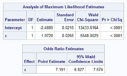
Notice that the estimated model parameters are close to the true parameters of -2.5 and 2. By default, the estimated odds ratio for a one unit increase in the predictor, Z, is provided. Under this model, a one unit increase in log(X) increases the event odds by about 7.2. Since Z is not involved in any interactions, the odds ratio of Z is constant, not depending on the value of Z. Using the data table above, subtracting the log odds at Z=0 (-2.5) from the log odds at Z=1.01 (-0.48) and exponentiating gives a rough estimate (7.54) for the true odds ratio of Z, and this estimate is similar to the 7.2 estimate from the fitted model:

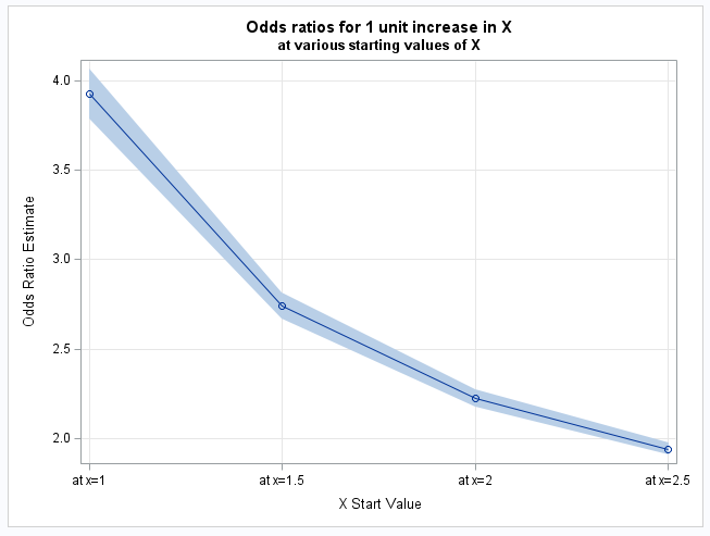
To estimate the odds ratios for one unit increases in X, rather one unit increases in Z, use the NLEST macro to evaluate the model at X and at X+1 and compute the odds ratios at various values of X. These evaluations are predicted log odds, so differencing and then exponentiating provide estimates of the odds ratios. This is most easily done by creating a data set with each of the expressions to be evaluated as shown below for X=1, 1.5, 2, and 2.5. To obtain a test that each odds ratio equals one (no change in odds) rather than zero as done by default, specify null=1 in the NLEST call. The macro automatically provides the same information as displayed in a data set named EST. Using that data set, PROC SGPLOT is used to plot the odds ratios and their confidence intervals:

   data fd; 
      length label f $32767; 
      infile datalines delimiter=',';
      input label f; 
      datalines;
   at x=1   , exp( (b_p1+log(1+1)*b_p2) - (b_p1+log(1)*b_p2) )
   at x=1.5 , exp( (b_p1+log(1.5+1)*b_p2) - (b_p1+log(1.5)*b_p2) )
   at x=2   , exp( (b_p1+log(2+1)*b_p2) - (b_p1+log(2)*b_p2) )
   at x=2.5 , exp( (b_p1+log(2.5+1)*b_p2) - (b_p1+log(2.5)*b_p2) )
   ;
   %nlest(instore=log, fdata=fd, null=1, title=ORs at various X values)

   proc sgplot data=est noautolegend;
      band upper=upper lower=lower x=label;
      series y=estimate x=label;
      scatter y=estimate x=label;
      yaxis grid label="Odds Ratio Estimate";
      xaxis grid label="X Start Value";
      title "Odds ratios for 1 unit increase in X";
      title2 "at various starting values of X";
      run;

Note the similarity of the estimated odds ratios to the true values in the data table above and how the odds ratios decrease when computed starting at larger values of X. As you can see in the data table above, a one unit increase is much larger in Z than in X, so the change in odds for a one unit increase can be expected to be much larger for Z than for X:

__________________

Note: In a model with log(X) as a predictor, you might intuitively think that the effect of a u=5 unit increase in X is βlog(5). However, consider again the simple linear model, E(Y) = α+βZ = α+βlog(X) and note the models that are being compared to arrive at this estimate. If you assess the effect of increasing Z by log(5) units, you would compare the models α+β[log(X)+log(5)] and α+βlog(X). Their difference is βlog(5). But notice that log(X)+log(5) = log(5X). So, rather than estimating the effect of increasing X by 5 units, βlog(5) actually estimates the effect of multiplying X by 5. As mentioned above, it also estimates the effect of increasing Z, not X, by log(5) = 1.61 units. If either of these last two estimates is of interest, it could be obtained using an ESTIMATE statement for a model with the identity link:

      estimate 'Mean Diff for 5X or Z+5' z 1.61;

For a logistic model, a similar statement estimates the odds ratio:

      estimate 'Odds ratio for 5X or Z+5' z 1.61 / exp;

Of course, the NLEST macro could also be used for these and other generalized linear models and assessment statistics.

Operating System and Release Information

Product Family	Product	System	SAS Release
			Reported	Fixed*
SAS System	N/A	Aster Data nCluster on Linux x64
		DB2 Universal Database on AIX
		DB2 Universal Database on Linux x64
		Netezza TwinFin 32-bit SMP Hosts
		Netezza TwinFin 32bit blade
		Netezza TwinFin 64-bit S-Blades
		Netezza TwinFin 64-bit SMP Hosts
		Teradata on Linux
		Cloud Foundry
		64-bit Enabled AIX
		64-bit Enabled HP-UX
		64-bit Enabled Solaris
		ABI+ for Intel Architecture
		AIX
		HP-UX
		HP-UX IPF
		IRIX
		Linux
		Linux for AArch64
		Linux for x64
		Linux on Itanium
		OpenVMS Alpha
		OpenVMS on HP Integrity
		Solaris
		Solaris for x64
		Tru64 UNIX
		z/OS
		z/OS 64-bit
		IBM AS/400
		OpenVMS VAX
		N/A
		Android Operating System
		Apple Mobile Operating System
		Chrome Web Browser
		Macintosh
		Macintosh on x64
		Microsoft Windows 10
		Microsoft Windows 7
		Microsoft Windows 8 Enterprise 32-bit
		Microsoft Windows 8 Enterprise x64
		Microsoft Windows 8 Pro 32-bit
		Microsoft Windows 8 Pro x64
		Microsoft Windows 8 x64
		Microsoft Windows Server 2008 R2
		Microsoft Windows Server 2012 R2 Datacenter
		Microsoft Windows Server 2012 R2 Std
		Microsoft® Windows® for 64-Bit Itanium-based Systems
		Microsoft Windows Server 2003 Datacenter 64-bit Edition
		Microsoft Windows Server 2003 Enterprise 64-bit Edition
		Microsoft Windows XP 64-bit Edition
		Microsoft® Windows® for x64
		OS/2
		SAS Cloud
		Microsoft Windows 8.1 Enterprise 32-bit
		Microsoft Windows 8.1 Enterprise x64
		Microsoft Windows 8.1 Pro 32-bit
		Microsoft Windows 8.1 Pro x64
		Microsoft Windows 11
		Microsoft Windows 95/98
		Microsoft Windows 2000 Advanced Server
		Microsoft Windows 2000 Datacenter Server
		Microsoft Windows 2000 Server
		Microsoft Windows 2000 Professional
		Microsoft Windows NT Workstation
Microsoft Windows Server 2003 Datacenter Edition
Microsoft Windows Server 2003 Enterprise Edition
Microsoft Windows Server 2003 Standard Edition
Microsoft Windows Server 2003 for x64
Microsoft Windows Server 2008
Microsoft Windows Server 2008 for x64
Microsoft Windows Server 2012 Datacenter
Microsoft Windows Server 2012 Std
Microsoft Windows Server 2016
Microsoft Windows Server 2019
Microsoft Windows Server 2022
Microsoft Windows XP Professional
Windows 7 Enterprise 32 bit
Windows 7 Enterprise x64
Windows 7 Home Premium 32 bit
Windows 7 Home Premium x64
Windows 7 Professional 32 bit
Windows 7 Professional x64
Windows 7 Ultimate 32 bit
Windows 7 Ultimate x64
Windows Millennium Edition (Me)
Windows Vista
Windows Vista for x64

* For software releases that are not yet generally available, the Fixed Release is the software release in which the problem is planned to be fixed.

---

Type:	Usage Note
Priority:
Topic:	Analytics ==> Regression SAS Reference ==> Macro

Date Modified:	2024-06-19 15:32:03
Date Created:	2024-06-13 13:17:52