Usage Note 70756: Compare group slopes on a continuous predictor in a spline or polynomial effect
 |  |  |
SAS Note 70221 discussed how to estimate the effect of a continuous predictor when the predictor is represented in the model using a flexible spline or polynomial. This note introduces multiple groups into the model with the goal of comparing group slopes on the continuous predictor. Specifically, the model allows the fitted curve of the continuous predictor to be different for each group. This is done by including the interaction between the group variable and the continuous predictor in the model. The idea is the same as what was discussed in SAS Note 24177, which compares group slopes in the simpler case where the model allows the continuous predictor to have only a linear effect in each group. In that simpler case, the slope in each group and their difference do not change across the range of the continuous predictor (at least on the link scale in a generalized linear model). In the case discussed below in which the effect over the continuous predictor is nonlinear, the slopes of the group curves must be estimated and compared at specific settings of the continuous predictor.
For more detail about assessing the effect of a continuous predictor that is involved in interaction in various types of models, see SAS Note 67024.
There are two important considerations that affect the choice of tools to be used to estimate and compare group slopes in a generalized linear model.
- Whether the continuous predictor of interest appears in the model in a spline or a polynomial effect. For a polynomial model, marginal effects can be used. For a spline model, differences of LS-means differences can be used.
- Whether the linear model estimates the response mean directly, as when the identity link is used, or whether a function of the response mean is modeled, as when other links are used such as the log or logit. When modeling the mean directly, the ESTIMATE statement can be used as shown in the ordinary regression examples discussed in SAS Note 70221. The following examples show approaches for models not using the identity link, such as logistic models.
The examples below use the binary response data in the example titled "Generalized Additive Model with Binary Data" in the GAM procedure documentation. A generalized linear model using the logit link is fit to the data with the continuous StartVert variable (renamed to SV) in either a spline or a polynomial effect. Slopes on SV will be estimated and compared in two groups, AGE=0 and 1, created by dichotomizing the Age variable at its median using the following PROC RANK step:
   proc rank data=kyphosis out=k(rename=(startvert=sv)) groups=2;
      var age; label age='Age';
      run;
Slope Differences in a Polynomial Model using Marginal Effects
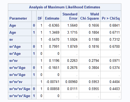
The following statements fit a logistic model with SV represented by separate cubic curves in each Age group. With the NOINT option to remove the overall intercept, the two Age parameters are the intercepts for the two Age groups. The first EFFECTPLOT statement shows the fitted curves on the logit (log odds) scale. The second EFFECTPLOT statement shows the curves on the event probability scale:
     proc logistic data=k;
        class age / param=glm;
        model kyphosis(event='1')=age|sv|sv|sv / noint;
        effectplot/noobs link;
        effectplot/noobs;
        run;
NOTE: The same cubic polynomial model can be fit using the EFFECT statement as follows, but the Margins macro does not accommodate models with constructed effects created using the EFFECT statement:
        effect p=polynomial(sv/degree=3);
        model kyphosis(event='1')=age|p / noint;
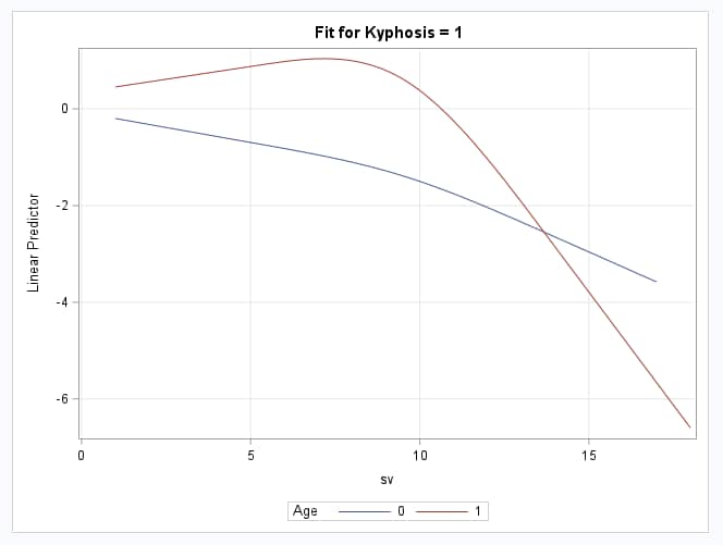
The results below show the parameters of the fitted model. Plots of the model on the link scale and then the probability scale are then shown. Note that the values of the Age intercepts appear consistent with the points at which the Age curves intercept at SV=0 on the link scale. Also note the distinctly different shapes of the two Age curves over SV:
   |
Suppose that it is of interest to compare the Age group slopes on SV. From the second plot above, it is clear that the complexity of the model allows for any nonlinearity in the association of SV with the event probability to show in the fitted curves. Because of this nonlinearity, the slope of each SV curve changes at different SV values. So, a comparison of the Age group slopes requires specifying the SV value at which the comparison is to be done. Suppose that comparison of slopes at SV values 5 and 10 are most of interest.
The following statements use the Margins macro (SAS Note 63038) to refit the above model (the macro used PROC GENMOD) and to then estimate the marginal effect of SV in each Age at both SV=5 and 10. As discussed more in SAS Note 22604, the marginal effect is the derivative of the curve at the specified point. So, it is the slope of a line drawn tangent to the curve at that point. It tells you the instantaneous rate of change in the event probability at the point.
To do the analysis, first create a simple data set, ATDAT, containing the two comparison points on SV in separate observations. The above model is respecified in the class= through modelopts= options. Estimation of marginal effects is specified by effect=sv and the inclusion of margins=age requests that the marginal effects be estimated in each Age level. To indicate the points on SV at which marginal effects are to be estimated, at=sv and atdata=atdat are specified. diff=all requests that the differences in marginal effects be computed and tested. Confidence intervals for the marginal effects and their difference are requested by options=cl. See the macro documentation (SAS Note 63038) for details about all available macro options:
     data atdat;
        do sv=5,10; output; end;
        run;
     %margins(data=k, class=age, response=kyphosis, roptions=event='1',
        model=age|sv|sv|sv, dist=binomial, modelopts=noint,
        margins=age, effect=sv, at=sv, atdata=atdat,
        diff=all, options=cl)
In the results from the macro, the Average Marginal Effects table provides the estimated slopes for each Age group at both SV=5 and 10. Note that the slope estimates are consistent with the apparent slopes at SV=5 and 10 in the above plot on the probability scale. The Differences table then provides the estimated difference in slopes (Age 0 - Age 1). The previous tables (not shown) of predictive margins and differences give the estimated event probabilities and differences for each Age group at SV=5 and 10:
  |
Slope Differences in a Spline Model using Differences of Differences
An alternative to using a polynomial to represent the effect of SV is to use a spline instead. Splines are very flexible effects that are not as limited in shape as polynomials. Notice in the above plots how the polynomial forces the fitted curves to rebend outward as they approach SV=0. Unlike a polynomial, a spline can flatten in regions as dictated by the data. A spline effect can be created using the EFFECT statement in many procedures including PROC LOGISTIC. For more information about splines and their construction, see the description of the EFFECT statement in the Shared Concepts and Topics chapter in the SAS/STAT User's Guide. Also, see SAS Notes 70221 and 67024.
Since the Margins macro does not accommodate constructed effects, such as splines, a different approach can be taken to estimate the slopes on SV at certain places on the curves. Using the well-known idea of slope as rise/run, the slope can be estimated as the difference in values spaced one unit apart (or by dividing the difference by the number of units spanned). LSMEANS statements can be used to obtain the appropriate coefficients of the model parameters to estimate the response at 5 and 6 and also at 10 and 11. Note that the LSMEANS statement requires use of GLM coding for CLASS variables. The NLMeans macro (SAS Note 62362) can then be used to estimate the slope on the mean (probability) scale across those pairs of points.
The following statements use the EFFECT statement to create a natural cubic spline for the SV variable. The spline effect, S, is then used in the model interacting with Age in the same way as done for the polynomial model above. The model is saved using the STORE statement. The EFFECTPLOT statements plot the fitted spline model on both the link (log odds) and probability scale as done for the polynomial model. The LSMEANS statements estimate the log odds and, with the ILINK option, the event probability at each of the four points on SV. The coefficients on the parameters are saved in data set C:
   proc logistic data=k;
      class age / param=glm;
      effect s=spline(sv/naturalcubic);
      model kyphosis(event='1')=age age*s / noint;
      lsmeans age/at sv=5 ilink e;
      lsmeans age/at sv=6 ilink e;
      lsmeans age/at sv=10 ilink e;
      lsmeans age/at sv=11 ilink e;
      effectplot/noobs;
      effectplot/noobs link;
      store kmod;
      ods output coef=c;
      run;
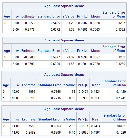
In the plots of the model, note the much more straight line shape of the curves as they approach SV=0. The Least Squares Means tables provide the estimated log odds (Estimate column) and event probabilities (Mean column) for each Age at each of the four SV points:
    |
To estimate the slopes on the probability scale from 5 to 6 and 10 to 11, contrasts of the LS-means are computed by the NLMeans macro. The following DATA step defines contrasts that, for each Age, compute the differences (slopes) and then the difference of those differences, which is the difference in slopes. The comments below the columns of contrast coefficients label the columns to make interpreting each contrast easier to see. Note that the coefficients in each contrast are specified in the order in which the LS-means are presented in the displayed results from PROC LOGISTIC.
The NLMeans macro is then called using the saved model, parameter coefficients, and contrast coefficients to make the computations. link=logit tells the macro the link function (logit) used in the model, and options=joint is needed so that the contrasts can be applied across all of the LSMEANS statement results. See the macro documentation (SAS Note 62362) for details about all available macro options:
   data difdif;
      input label & $25. k1-k8;
      set=1;
      datalines;
   SV6-SV5 in Age0         -1  0    1  0    0  0    0  0
   SV6-SV5 in Age1          0 -1    0  1    0  0    0  0
   SV6-SV5 in Age1-Age0     1 -1   -1  1    0  0    0  0
   SV11-SV10 in Age0        0  0    0  0   -1  0    1  0
   SV11-SV10 in Age1        0  0    0  0    0 -1    0  1
   SV11-SV10 in Age1-Age0   0  0    0  0    1 -1   -1  1
   ;             /*         ----    ----    ----    ----  */
                 /*    AGE: 0  1    0  1    0  1    0  1  */
                 /*     SV:   5       6      10      11   */

   %nlmeans(instore=kmod, coef=c, contrasts=difdif, link=logit,
            options=joint, title=Risk differences at 5 and 10 for each Age)
The estimated slopes in each Age, computed as one unit risk differences from 5 to 6 and from 10 to 11, are displayed by the macro. Also the slope differences between Ages are given. Significance tests and confidence intervals are shown for each estimate. The estimates are consistent with the fitted curves in the plot on the probability scale above. Notice that the slope from SV=5 to SV=6 in Age=0 is negative but is positive in Age=1. The difference in slopes is estimated to be about 0.048. From SV=10 to SV=11, the slopes in both Ages are negative with the slope in Age=1 clearly more strongly negative. The slope difference is estimated to be about -0.121:
 |
Operating System and Release Information
| Product Family | Product | System | SAS Release | |
| Reported | Fixed* | |||
| SAS System | SAS/STAT | z/OS | ||
| z/OS 64-bit | ||||
| OpenVMS VAX | ||||
| Microsoft® Windows® for 64-Bit Itanium-based Systems | ||||
| Microsoft Windows Server 2003 Datacenter 64-bit Edition | ||||
| Microsoft Windows Server 2003 Enterprise 64-bit Edition | ||||
| Microsoft Windows XP 64-bit Edition | ||||
| Microsoft® Windows® for x64 | ||||
| OS/2 | ||||
| Microsoft Windows 8 Enterprise 32-bit | ||||
| Microsoft Windows 8 Enterprise x64 | ||||
| Microsoft Windows 8 Pro 32-bit | ||||
| Microsoft Windows 8 Pro x64 | ||||
| Microsoft Windows 8.1 Enterprise 32-bit | ||||
| Microsoft Windows 8.1 Enterprise x64 | ||||
| Microsoft Windows 8.1 Pro 32-bit | ||||
| Microsoft Windows 8.1 Pro x64 | ||||
| Microsoft Windows 10 | ||||
| Microsoft Windows 11 | ||||
| Microsoft Windows 95/98 | ||||
| Microsoft Windows 2000 Advanced Server | ||||
| Microsoft Windows 2000 Datacenter Server | ||||
| Microsoft Windows 2000 Server | ||||
| Microsoft Windows 2000 Professional | ||||
| Microsoft Windows NT Workstation | ||||
| Microsoft Windows Server 2003 Datacenter Edition | ||||
| Microsoft Windows Server 2003 Enterprise Edition | ||||
| Microsoft Windows Server 2003 Standard Edition | ||||
| Microsoft Windows Server 2003 for x64 | ||||
| Microsoft Windows Server 2008 | ||||
| Microsoft Windows Server 2008 R2 | ||||
| Microsoft Windows Server 2008 for x64 | ||||
| Microsoft Windows Server 2012 Datacenter | ||||
| Microsoft Windows Server 2012 R2 Datacenter | ||||
| Microsoft Windows Server 2012 R2 Std | ||||
| Microsoft Windows Server 2012 Std | ||||
| Microsoft Windows Server 2016 | ||||
| Microsoft Windows Server 2019 | ||||
| Microsoft Windows Server 2022 | ||||
| Microsoft Windows XP Professional | ||||
| Windows 7 Enterprise 32 bit | ||||
| Windows 7 Enterprise x64 | ||||
| Windows 7 Home Premium 32 bit | ||||
| Windows 7 Home Premium x64 | ||||
| Windows 7 Professional 32 bit | ||||
| Windows 7 Professional x64 | ||||
| Windows 7 Ultimate 32 bit | ||||
| Windows 7 Ultimate x64 | ||||
| Windows Millennium Edition (Me) | ||||
| Windows Vista | ||||
| Windows Vista for x64 | ||||
| 64-bit Enabled AIX | ||||
| 64-bit Enabled HP-UX | ||||
| 64-bit Enabled Solaris | ||||
| ABI+ for Intel Architecture | ||||
| AIX | ||||
| HP-UX | ||||
| HP-UX IPF | ||||
| IRIX | ||||
| Linux | ||||
| Linux for x64 | ||||
| Linux on Itanium | ||||
| OpenVMS Alpha | ||||
| OpenVMS on HP Integrity | ||||
| Solaris | ||||
| Solaris for x64 | ||||
| Tru64 UNIX | ||||
| Type: | Usage Note |
| Priority: | |
| Topic: | Analytics ==> Regression SAS Reference ==> Macro |
| Date Modified: | 2024-04-16 09:50:49 |
| Date Created: | 2024-04-15 16:45:54 |