Usage Note 69873: Estimate the predictor value yielding a specified response value
 |  |  |
When using a regression method to fit a model to data, one of the most common goals is to use that model to estimate the response mean, μ, for a given setting of the predictor variables in the model. However, the reverse of this goal is sometimes of interest – that is, to estimate the value of a predictor variable that yields a particular response value while holding the other predictors in the model, if any, at fixed values. This is sometimes referred to as calibration or inverse regression.
Consider a generalized linear model
g(μ) = Xβ ,
where g(·) is a link function, X is the model matrix of predictor settings, and β are the model parameters to be estimated. Suppose you want to estimate the value of the X1 predictor yielding a response mean value of μ1. Rewrite the model as
g(μ) = β1x1 + X*β* ,
where X*β* is the portion of the model matrix and parameter vector omitting x1 and its parameter, β1. Note that this includes the intercept column and parameter if present in the model.
Solving for x1
x1 = (g(μ) - X*β*) / β1 .
So, an estimate of the x1 value yielding response mean μ1 is
^ x1 = (g(μ1) - X* ^ β* ) / ^ β1 .
Note that this estimator is a ratio of random values with model parameters in both the numerator and the denominator. While a point estimate for x1 is easily produced using the estimated model parameters, obtaining a standard error and confidence interval is not so straightforward. Since this is a nonlinear function of the model parameters, the ESTIMATE statement that is available in many modeling procedures cannot be used since it estimates only linear functions. However, you can use the NLEST macro (SAS Note 58775) to estimate nonlinear functions. If you fit the model using the NLMIXED procedure, it can also be done using the ESTIMATE statement in that procedure, which is not restricted to linear functions. With either approach, the standard error is estimated using the delta method.
For binary response models such as logistic and probit models, inverse regression estimates can be obtained more simply by fitting the model in the PROBIT procedure and using the INVERSECL option. Examples can be found in SAS Note 44931 and at the end of SAS Note 56476. Also see the examples in the PROBIT procedure documentation titled "Dosage Levels" and "An Epidemiology Study."
Normal Response Model with Interaction
Consider the following model for a normally distributed response variable, Y, as a function of X1, X2, and their interaction. For this ordinary regression model, the link function is the identity link, g(μ)=μ.
μ = β0 + β1x1 + β2x2 + β3x1x2
Rewrite the model as
μ = β0 + (β1 + β3x2) x1 + β2x2 .
Then the estimate of x1 yielding a response mean of μ1 is
^ x1 = (μ1 - ^ β0 - ^ β2 x2) / ( ^ β1 + ^ β3 x2 ) .
The following statements generate data from the model using known parameter values as shown. TrueX1at50 computes the actual value of X1, under this model, that produces a mean value of Y equal to 50 in each observation. This value changes only as x2 changes.
     data a;
        call streaminit(23422);
        scale=10;
        do x1=1 to 10;
         do x2=1 to 5;
          do n=1 to 1000;
            mean=10 + 5*x1 - 2*x2 + 0.5*x1*x2;
            std=scale;
            TrueX1at50 = (50-10+2*x2)/(5+0.5*x2);
            y=rand('normal',mean,scale);
            output;
          end;
         end;
        end;
        run;
These statements fit the normal response model with interaction using the GENMOD procedure, though other regression procedures could be used. The EFFECTPLOT statement shows the predicted values from the model as a set of lines for the values of x2. The OUTPUT statement saves the predicted values in data set OUT. The STORE statement saves the fitted model in an item store named GEN. This will be used the NLEST macro.
     proc genmod data=a;
        model y=x1|x2;
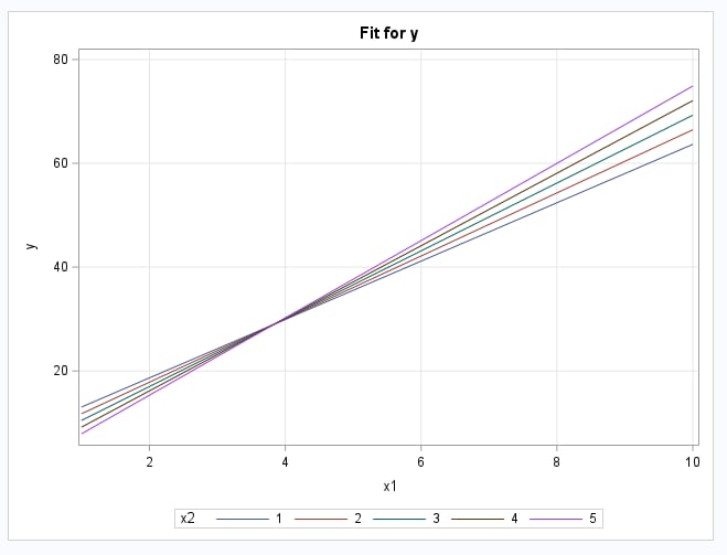
        effectplot slicefit(x=x1 sliceby=x2);
        output out=out p=p;
        store gen;
        run;
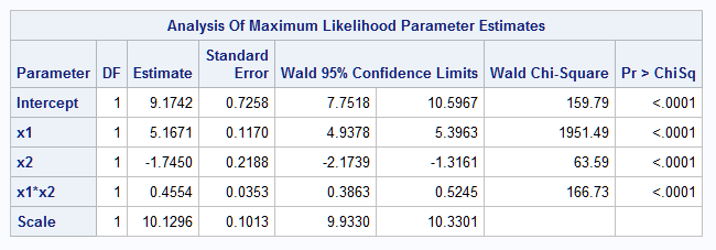
The following shows the fitted model parameters. Note that they closely match the true model specified in the DATA step code above. The fitted model is displayed in the plot that follows.
  |
The NLEST macro is called to estimate the nonlinear function of model parameters as shown above. Note that the macro uses names for the model parameters of the form B_P1, B_P2, and so on in the order provided by the modeling procedure. Since the function involves the x2 values, score=a is specified so that the macro estimates the function for each observation in data set A. When score= is specified, the default output data set produced by the macro is named NLEST.
%nlest(instore=gen, f=(50-b_p1-b_p3*x2)/(b_p2+b_p4*x2), score=a)
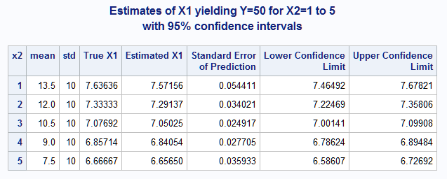
These statements display the estimated values of x1 that yield a response mean of 50 for each value of x2 along with their standard errors and 95% large-sample confidence intervals. The SORT step simply keeps one observation per x2 value since all observations with the same x2 value have the sample estimate.
     proc sort data=nlest out=nlest2 nodupkey;
        by x2;
        run;
     proc print data=nlest2 label;
        id x2;
        var mean std TrueX1at50 pred stderrpred lower upper;
        label TrueX1at50="True X1" pred="Estimated X1";
        title "Estimates of X1 yielding Y=50 for X2=1 to 5";
        title2 "with 95% confidence intervals";
        run;
Note that the x1 values yielding Y=50 estimated using the generated data closely match the actual values (True X1) under the specified model.
 |
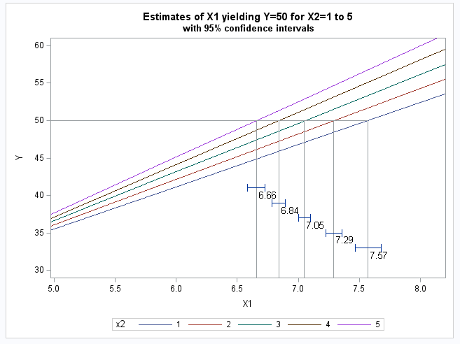
The following statements produce a plot showing the fitted model, the estimated x1 values and their confidence intervals.
     data nlest2; set nlest2;
        pos=30+2*_n_; pos2=pos+1;
        predval=" "||put(pred,4.2);
        run;
     data out2; set out nlest2(keep=pos pred predval x2 pos2 lower upper); run;
     proc sgplot;
        series y=p x=x1 / group=x2;
        dropline y=50 x=pred / dropto=both;
        text x=pred y=pos text=predval / position=right textattrs=(size=10);
        highlow y=pos2 low=lower high=upper / lowcap=serif highcap=serif;
        xaxis min=5 max=8 label="X1";
        yaxis min=30 max=60 label="Y";
        run;
 |
The same estimates can be produced by fitting the model in the NLMIXED procedure. These statements fit the model and use the PREDICT statement to estimate the x1 values yielding Y=50. The ESTIMATE statement cannot be used since the function involves values in the data. The same estimated values, standard errors, and confidence intervals as shown above are computed and saved in data set EST for each observation.
     proc nlmixed data=a df=1e8;
        mean = b0 + b1*x1 + b2*x2 + b3*x1*x2;
        model y ~ normal(mean,s**2);
        predict (50-b0-b2*x2)/(b1+b3*x2) out=est;
        run;
Gamma Response Model
The same process can be used for generalized linear models involving other response distributions. The following DATA step generates response values from the gamma distribution as a function of a single predictor, x. The generating model uses the log link function. The model is
log(μ) = β0 + β1x
The goal is to estimate the value of x that produces a mean response of μ=6. Using the above formula, the actual value of x yielding a mean of 6 is (log(6)-1)/0.15 = 5.28.
     data a;
        call streaminit(23422);
        scale=.5;
        do x=1 to 10;
         do n=1 to 100;
           mean=exp(1 + 0.15*x);
           lambda=mean/scale;
           std=sqrt(mean**2/scale);
           y=rand('gamma',scale,lambda);
           output;
         end;
        end;
        run;
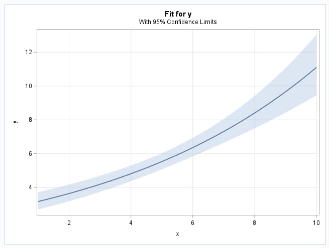
The GENMOD procedure is again used to fit the model although another procedure could be used. The fitted model is plotted and saved and the predicted values are saved in a data set.
     proc genmod data=a;
        model y = x / dist=gamma link=log;
        output out=out p=p;
        effectplot;
        store gen;
        run;
The parameter estimates of the fitted model closely agree with the true parameters specified in the generating model above.
  |
Since there is only one predictor in the model, there is only a single estimate of the value producing the desired response. In this case, you can simply specify the desired function in f= in the NLEST macro. Optionally, you can specify a label for the estimate in label=. If the predictor value for more than one response mean is to be estimated, you can create a data set containing all of the function expressions and then specify that data set in fdata=. You can see examples using fdata= in the NLEST macro documentation (SAS Note 58775). By default, the result from the macro are saved in a data set named EST.
%nlest(instore=gen, label=X: Y=6, f=(log(6)-b_p1)/b_p2)
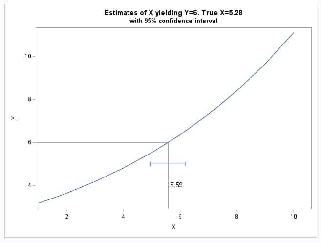
The result displayed by the macro shows that the estimate of x that produces a response mean of 6 is 5.59 with 95% large-sample confidence interval (4.97,6.20). The point estimate is slightly off from the true value of 5.28 due to sampling error, but it is well within the confidence interval.
 |
These statements replot the model and add the estimate of x and its confidence interval.
     data out2; set out est;
        pos=4; pos2=pos+1;
        predval=" "||put(estimate,4.2);
        run;
     proc sgplot noautolegend;
        series y=p x=x;
        dropline y=6 x=estimate / dropto=both;
        text x=estimate y=pos text=predval / position=right textattrs=(size=10);
        highlow y=pos2 low=lower high=upper / lowcap=serif highcap=serif;
        xaxis label="X";
        yaxis label="Y";
        title "Estimates of X yielding Y=6. True X=5.28";
        title2 "with 95% confidence interval";
        run;
 |
Again, the same estimates can be produced by fitting the model in the NLMIXED procedure. Since the function estimate does not involve any data values from other predictors, the ESTIMATE statement can be used. The following statements produce the same estimated values, standard errors and confidence intervals as shown above.
     proc nlmixed data=a df=1e8;
        mean=exp(b0+b1*x);
        lambda=mean/s;
        model y ~ gamma(s,lambda);
        estimate 'x:y=6' (log(6)-b0)/b1;
        run;
Operating System and Release Information
| Product Family | Product | System | SAS Release | |
| Reported | Fixed* | |||
| SAS System | N/A | Netezza TwinFin 64-bit SMP Hosts | ||
| Teradata on Linux | ||||
| Solaris | ||||
| Solaris for x64 | ||||
| OpenVMS on HP Integrity | ||||
| OpenVMS Alpha | ||||
| Cloud Foundry | ||||
| 64-bit Enabled AIX | ||||
| 64-bit Enabled HP-UX | ||||
| 64-bit Enabled Solaris | ||||
| ABI+ for Intel Architecture | ||||
| AIX | ||||
| HP-UX | ||||
| HP-UX IPF | ||||
| IRIX | ||||
| Linux | ||||
| Linux for AArch64 | ||||
| Linux for x64 | ||||
| Linux on Itanium | ||||
| Netezza TwinFin 64-bit S-Blades | ||||
| Netezza TwinFin 32bit blade | ||||
| Netezza TwinFin 32-bit SMP Hosts | ||||
| DB2 Universal Database on Linux x64 | ||||
| DB2 Universal Database on AIX | ||||
| Aster Data nCluster on Linux x64 | ||||
| Tru64 UNIX | ||||
| z/OS | ||||
| z/OS 64-bit | ||||
| IBM AS/400 | ||||
| OpenVMS VAX | ||||
| N/A | ||||
| Android Operating System | ||||
| Apple Mobile Operating System | ||||
| Chrome Web Browser | ||||
| Macintosh | ||||
| Macintosh on x64 | ||||
| Microsoft Windows 10 | ||||
| Microsoft Windows 7 | ||||
| Microsoft Windows 8 Enterprise 32-bit | ||||
| Microsoft Windows 8 Enterprise x64 | ||||
| Microsoft Windows 8 Pro 32-bit | ||||
| Microsoft Windows 8 Pro x64 | ||||
| Microsoft Windows 8 x64 | ||||
| Microsoft Windows Server 2008 R2 | ||||
| Microsoft Windows Server 2012 R2 Datacenter | ||||
| Microsoft Windows Server 2012 R2 Std | ||||
| Microsoft® Windows® for 64-Bit Itanium-based Systems | ||||
| Microsoft Windows Server 2003 Datacenter 64-bit Edition | ||||
| Microsoft Windows Server 2003 Enterprise 64-bit Edition | ||||
| Microsoft Windows XP 64-bit Edition | ||||
| Microsoft® Windows® for x64 | ||||
| OS/2 | ||||
| SAS Cloud | ||||
| Microsoft Windows 8.1 Enterprise 32-bit | ||||
| Microsoft Windows 8.1 Enterprise x64 | ||||
| Microsoft Windows 8.1 Pro 32-bit | ||||
| Microsoft Windows 8.1 Pro x64 | ||||
| Microsoft Windows 11 | ||||
| Microsoft Windows 95/98 | ||||
| Microsoft Windows 2000 Advanced Server | ||||
| Microsoft Windows 2000 Datacenter Server | ||||
| Microsoft Windows 2000 Server | ||||
| Microsoft Windows 2000 Professional | ||||
| Microsoft Windows NT Workstation | ||||
| Microsoft Windows Server 2003 Datacenter Edition | ||||
| Microsoft Windows Server 2003 Enterprise Edition | ||||
| Microsoft Windows Server 2003 Standard Edition | ||||
| Microsoft Windows Server 2003 for x64 | ||||
| Microsoft Windows Server 2008 | ||||
| Microsoft Windows Server 2008 for x64 | ||||
| Microsoft Windows Server 2012 Datacenter | ||||
| Microsoft Windows Server 2012 Std | ||||
| Microsoft Windows Server 2016 | ||||
| Microsoft Windows Server 2019 | ||||
| Microsoft Windows Server 2022 | ||||
| Microsoft Windows XP Professional | ||||
| Windows 7 Enterprise 32 bit | ||||
| Windows 7 Enterprise x64 | ||||
| Windows 7 Home Premium 32 bit | ||||
| Windows 7 Home Premium x64 | ||||
| Windows 7 Professional 32 bit | ||||
| Windows 7 Professional x64 | ||||
| Windows 7 Ultimate 32 bit | ||||
| Windows 7 Ultimate x64 | ||||
| Windows Millennium Edition (Me) | ||||
| Windows Vista | ||||
| Windows Vista for x64 | ||||
| Type: | Usage Note |
| Priority: | |
| Topic: | Analytics ==> Regression SAS Reference ==> Macro SAS Reference ==> Procedures ==> NLMIXED SAS Reference ==> Procedures ==> GENMOD |
| Date Modified: | 2023-02-17 15:55:56 |
| Date Created: | 2023-02-16 11:28:24 |