Usage Note 69066: The effect of time in repeated measures analysis in the MIXED procedure
 |  |  |
When you have repeated measures data and the response variable is assumed normal, you typically use PROC MIXED to analyze the data. One of the possible models is to use the REPEATED statement in PROC MIXED to model the correlations in your data. However, with different data situations for your TIME variable, and different model specifications in your PROC MIXED program, the results might not be what you expect, as explained below for three scenarios.
The repeated measures data comes from the example titled "Repeated Measures" in the PROC MIXED documentation. The name of the time variable is changed from Age to Time for clarity.
     data pr;
        input Person Gender $ y1 y2 y3 y4;
        y=y1; Time=8;  output;
        y=y2; Time=10; output;
        y=y3; Time=12; output;
        y=y4; Time=14; output;
        drop y1-y4;
        datalines;
     1    F   21.0    20.0    21.5    23.0
     2    F   21.0    21.5    24.0    25.5
     3    F   20.5    24.0    24.5    26.0
     4    F   23.5    24.5    25.0    26.5
     5    F   21.5    23.0    22.5    23.5
     6    F   20.0    21.0    21.0    22.5
     7    F   21.5    22.5    23.0    25.0
     8    F   23.0    23.0    23.5    24.0
     9    F   20.0    21.0    22.0    21.5
     10   F   16.5    19.0    19.0    19.5
     11   F   24.5    25.0    28.0    28.0
     12   M   26.0    25.0    29.0    31.0
     13   M   21.5    22.5    23.0    26.5
     14   M   23.0    22.5    24.0    27.5
     15   M   25.5    27.5    26.5    27.0
     16   M   20.0    23.5    22.5    26.0
     17   M   24.5    25.5    27.0    28.5
     18   M   22.0    22.0    24.5    26.5
     19   M   24.0    21.5    24.5    25.5
     20   M   23.0    20.5    31.0    26.0
     21   M   27.5    28.0    31.0    31.5
     22   M   23.0    23.0    23.5    25.0
     23   M   21.5    23.5    24.0    28.0
     24   M   17.0    24.5    26.0    29.5
     25   M   22.5    25.5    25.5    26.0
     26   M   23.0    24.5    26.0    30.0
     27   M   22.0    21.5    23.5    25.0
     ;
The following statements fit the model to be used throughout.
     proc mixed data=pr ;
        class Person Gender Time;
        model y = Gender Time Gender*Time / s;
        repeated Time / type=ar(1) subject=Person r;
     run;
Following is partial output.
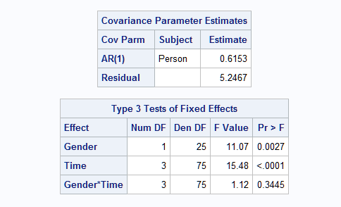 |
1. Missing Values for Some Time Points
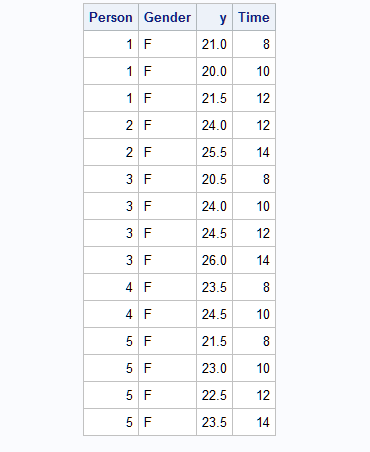
The PR data set is balanced in that each subject has four repeated measures at time values of 8, 9, 10, and 11. Now suppose that not every subject has all four repeated measures, as in data set NEW, and the model is refitted.
     data new;
       set pr;
       if _n_ in (4,5,6,15,16,26) then delete;
     run;

     proc mixed data=new ;
        class Person Gender Time;
        model y = Gender Time Gender*Time / s;
        repeated Time / type=ar(1) subject=Person r;
     run;
Partial results that reflect the change in the data are shown below:
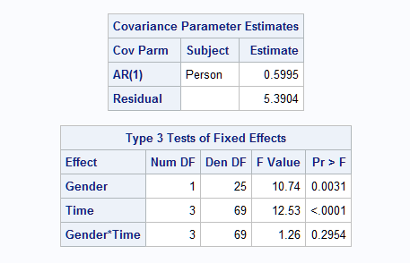 |
However, if you do not specify the repeated effect, TIME, in the REPEATED statement, you get different and incorrect results that might be unexpected.
     proc mixed data=new ;
        class Person Gender Time;
        model y = Gender Time Gender*Time / s;
        repeated / type=ar(1) subject=Person r;
     run;
Here are the results from this analysis.
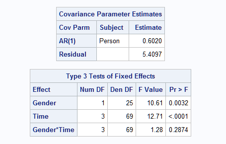 |
The reason the two approaches produce different results is that without the TIME effect in the REPEATED statement, the repeated measures for subjects are treated differently. To explain this problem, examine the first few observations in data set NEW.
 |
For subject 2, the repeated measures are considered the second and fourth time points for the model when the repeated effect, TIME, is in the REPEATED statement. However, they are considered the first and second time points when TIME is not specified as the repeated effect in the REPEATED statement. Therefore, it is recommended that you specify the repeated effect whenever possible in the REPEATED statement in PROC MIXED.
2. Specifying the REF= Option for TIME in the CLASS Statement
You can specify the REF= option in the CLASS statement so that the "Solutions for Fixed Effects" table produces the differences with the desired reference level. However, this option can cause the repeated measures to be sorted in a different order and therefore produce unexpected results. That is illustrated below.
     proc mixed data=pr ;
        class Person Gender Time(ref='8');
        model y = Gender Time Gender*Time / s;
        repeated Time / type=ar(1) subject=Person r;
     run;
Partial output follows.
 |
Note that in PROC MIXED (also in the GLM and GLIMMIX procedures), specifying the reference category essentially reorders the levels for the CLASS variable. In this case, the order for TIME is 10 12 14 8. So the observation for time 8 is considered the last time point and that affects the estimation of the AR(1) parameters. The results are also affected as shown below.
 |
It is recommended that you do not use the REF= option to change the order of the levels of the TIME variable unless the change creates the proper chronological order.
If you want to compare the mean response at different time points against a certain time point, you can use the LSMEANS statement with the DIFF=CONTROL option to specify the desired reference time level.
lsmeans time / diff=control('8');
If you need to use TIME='8' as the reference level but still preserve the natural order of time for the AR(1) covariance structure, you can create a duplicate TIME variable, such as TIME1, and use TIME1 as the REPEATED effect. Here is an example:
     data pr;
        set pr;
        Time1=Time;
     run;
     proc mixed data=pr ;
        class Person Gender Time(ref='8') Time1;
        model y = Gender Time Gender*Time / s;
        repeated Time1 / type=ar(1) subject=Person r;
     run;
3. Appending New Observations to Obtain Predicted Values for Them
As discussed in SAS Note 33307 on scoring new observations, the following restates method 3 ("Augment the Training Data Set"), which is often used to score (obtain predicted values for) new observations. This approach works with many modeling procedures.
- Create a scoring data set with values for all independent variables in your model and the values for which you want to obtain predicted values. The values for the response variable are all set to missing.
- Append this scoring data set to the original data set.
- Run your model using this combined data set and use the appropriate statement or option to obtain predicted values. In PROC MIXED, use the OUTP= option in the MODEL statement to obtain a data set of predicted values.
Note, however, that with this or any other scoring method, the predicted value for a new observation can still be missing for a number of reasons – the most typical being that the value of a variable involved in fitting the model is missing or invalid, or that the value of a CLASS variable (other than the SUBJECT= variable) is not one seen in the observations used to fit the model. These and other possible reasons are detailed in SAS Note 32304.
Because the observations in the scoring data set have missing values for the response variable, they are not used in the model estimation process. The model results are therefore unaffected, but by including these observations in the data set, predicted values are computed for these observations. However, situations can be complex for the TIME variable in a repeated measures analysis. This is illustrated below.
Suppose it is of interest to consider the linear effect of TIME rather than differences among the four specific time points that appear in the data. This implies removing TIME from the CLASS statement so that it is treated as a continuous predictor in the model. Since TIME is also used in the REPEATED statement and therefore must be a CLASS variable, you can, as above, create a copy of the TIME variable (TIME1) to use as a classification repeated effect in the REPEATED statement.
Additionally, suppose that estimates at some intermediate times are wanted. These statements create the TIME1 copy of the TIME variable in the PR data set and a data set of the additional predictor settings to score:
     data pr;
        set pr;
        Time1=Time;
        run;
     data scoring;
       input person gender $ time y;
       datalines;
       1  F 8.5 .
       13 M 9.5 .
       30 F 10  .
       ;
One approach for computing predicted values is to use the STORE statement in PROC MIXED to save the fitted model and then use the SCORE statement in the PLM procedure to obtain the predicted values as shown below. Note that, as described above, TIME appears in the MODEL statement but not in the CLASS statement so that TIME is modeled as a continuous, linear effect. The TIME1 copy of TIME is specified in the CLASS statement so that it can be used in the SUBJECT= option in the REPEATED statement:
     proc mixed data=pr;
        class Person Gender Time1;
        model y = Gender Time Gender*Time / s;
        repeated Time1 / type=ar(1) subject=Person r;
        store mxout;
        run;
     proc plm restore=mxout;
        score data=scoring out=preddata2 predicted=pred;
        run;
     proc print data=preddata2;
        run;
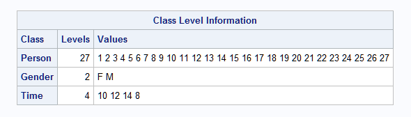
The scored additional observations are shown below. The Class Level Information table below shows that the analysis involved only the original four time points since time points 8.5 and 9.5 do not appear in the data used to fit the model. However, those two time points are used to compute predicted values based on the parameter estimates of the model with the linear effect of TIME:
   |
There are two points about PROC PLM that are worth mentioning:
- The predicted vales from PROC PLM will not be kriging predictions as is the case in the OUTP= data set with PROC MIXED. Instead, they will be the same predicted values as reported by the PROC GLIMMIX model with only a random R-side effect. If you want the kriging predictions, do not use PROC PLM.
- When you specify a RANDOM statement in PROC MIXED, the SCORE statement in PROC PLM does not compute the predicated values involving random effects. If you want the predicted values to include the random effects, consider using the LMIXED procedure with the STORE statement in SAS® Viya® to fit your mixed model. Then use the ASTORE procedure with the SCORE statement to obtain predicted values.
Another approach is to combine the original and scoring data, create a copy of the TIME variable as mentioned above, and refit the model. However, this has an effect on the model:
     data all;
        set pr scoring;
        time1=time;
        run;
     proc mixed data=all;
        class Person Gender Time1;
        model y = Gender Time Gender*Time / s outp=preddata2;
        repeated Time1 / type=ar(1) subject=Person r;
        run;
     proc print data=preddata2;
        run;
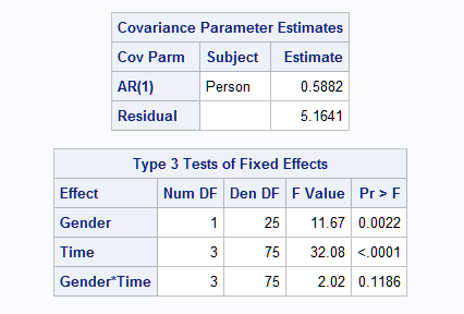
Note that the model results are different from the model above, which was fit only to the original data. This is because observations with TIME values 8.5 and 9.5 are added as shown in the Class Level Information table below. With the addition of these observations, the TIME values in the original data set (8, 10, 12, and 14) are now considered the first, fourth, fifth, and sixth time points when estimating the correlations in the repeated measures as specified in the REPEATED statement. The additional time points affect the results as shown in the table of Type 3 tests.
The predictions are now computed based on the new time points in the combined data set. If you intend for the model to use only the additional time points for scoring, but not to consider them when fitting the model, then you should use the approach using PROC PLM as above.
   |
Operating System and Release Information
| Product Family | Product | System | SAS Release | |
| Reported | Fixed* | |||
| SAS System | SAS/STAT | z/OS | ||
| z/OS 64-bit | ||||
| OpenVMS VAX | ||||
| Microsoft® Windows® for 64-Bit Itanium-based Systems | ||||
| Microsoft Windows Server 2003 Datacenter 64-bit Edition | ||||
| Microsoft Windows Server 2003 Enterprise 64-bit Edition | ||||
| Microsoft Windows XP 64-bit Edition | ||||
| Microsoft® Windows® for x64 | ||||
| OS/2 | ||||
| Microsoft Windows 8 Enterprise 32-bit | ||||
| Microsoft Windows 8 Enterprise x64 | ||||
| Microsoft Windows 8 Pro 32-bit | ||||
| Microsoft Windows 8 Pro x64 | ||||
| Microsoft Windows 8.1 Enterprise 32-bit | ||||
| Microsoft Windows 8.1 Enterprise x64 | ||||
| Microsoft Windows 8.1 Pro 32-bit | ||||
| Microsoft Windows 8.1 Pro x64 | ||||
| Microsoft Windows 10 | ||||
| Microsoft Windows 11 | ||||
| Microsoft Windows 95/98 | ||||
| Microsoft Windows 2000 Advanced Server | ||||
| Microsoft Windows 2000 Datacenter Server | ||||
| Microsoft Windows 2000 Server | ||||
| Microsoft Windows 2000 Professional | ||||
| Microsoft Windows NT Workstation | ||||
| Microsoft Windows Server 2003 Datacenter Edition | ||||
| Microsoft Windows Server 2003 Enterprise Edition | ||||
| Microsoft Windows Server 2003 Standard Edition | ||||
| Microsoft Windows Server 2003 for x64 | ||||
| Microsoft Windows Server 2008 | ||||
| Microsoft Windows Server 2008 R2 | ||||
| Microsoft Windows Server 2008 for x64 | ||||
| Microsoft Windows Server 2012 Datacenter | ||||
| Microsoft Windows Server 2012 R2 Datacenter | ||||
| Microsoft Windows Server 2012 R2 Std | ||||
| Microsoft Windows Server 2012 Std | ||||
| Microsoft Windows Server 2016 | ||||
| Microsoft Windows Server 2019 | ||||
| Microsoft Windows Server 2022 | ||||
| Microsoft Windows XP Professional | ||||
| Windows 7 Enterprise 32 bit | ||||
| Windows 7 Enterprise x64 | ||||
| Windows 7 Home Premium 32 bit | ||||
| Windows 7 Home Premium x64 | ||||
| Windows 7 Professional 32 bit | ||||
| Windows 7 Professional x64 | ||||
| Windows 7 Ultimate 32 bit | ||||
| Windows 7 Ultimate x64 | ||||
| Windows Millennium Edition (Me) | ||||
| Windows Vista | ||||
| Windows Vista for x64 | ||||
| 64-bit Enabled AIX | ||||
| 64-bit Enabled HP-UX | ||||
| 64-bit Enabled Solaris | ||||
| ABI+ for Intel Architecture | ||||
| AIX | ||||
| HP-UX | ||||
| HP-UX IPF | ||||
| IRIX | ||||
| Linux | ||||
| Linux for x64 | ||||
| Linux on Itanium | ||||
| OpenVMS Alpha | ||||
| OpenVMS on HP Integrity | ||||
| Solaris | ||||
| Solaris for x64 | ||||
| Tru64 UNIX | ||||
| Type: | Usage Note |
| Priority: | |
| Topic: | Analytics ==> Mixed Models Analytics ==> Regression Analytics ==> Scoring SAS Reference ==> Procedures ==> GLIMMIX SAS Reference ==> Procedures ==> MIXED |
| Date Modified: | 2026-02-19 10:14:17 |
| Date Created: | 2022-04-07 15:30:20 |