Sample 60856: Testing for Returns to Scale in a Cobb-Douglas Production Function
 |  |  |  |
Overview
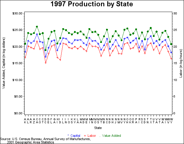
A production function is a function that summarizes the conversion of inputs in to outputs. For example, the production of cars using steel, labor, machinery, and plant facilities could be described as 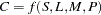 . Production functions can be applied to a single firm, an industry, or an entire nation. Note, however, that they are limited to producing a single output, so that joint production is disallowed, although multiple inputs are used. The simplest production function used frequently in economics is a Cobb-Douglas production function. This is a two-input production function that takes on the form
![\[ q = f(K,L) = AK^\alpha L^\beta \cdot e^\epsilon \]](http://support.sas.com/rnd/app/ets/examples/cobbdoug/images/ets_webex_cobbdoug0002.png) |
where output,  , is a function of two inputs, capital (
 ) and labor (
 ). The parameters
  and
and  are all positive constants calculated from empirical data and
  is a multiplicative exponential error. This type of production function is particularly useful since it is linear in logarithms and can be used to determine whether the inputs exhibit increasing, decreasing, or constant returns to scale. For example, suppose both the capital and the labor inputs are doubled. The Cobb-Douglas production function helps you determine what happens to the output. Will it also increase by double? Will output increase by more than double? Will it increase by some amount less than double?
Formally, for constant returns to scale,  . That is, if both of the inputs, capital and labor, are increased by a factor of
  , then output also increases by a factor of . For increasing returns, if both capital and labor are increased by a factor of , then output increases by an amount greater than . In this case,
  . The opposite is true for decreasing returns. If both capital and labor are increased by a factor of , then output increases by an amount less than such that
  .
.
The U.S. Census Bureau conducts an Annual Survey of Manufactures in each of the four years between the economic census. This survey is broken down into each of the 50 states and the District of Colombia in the 2001 Geographic Area Statistics. The data consist of labor hours as the estimate for labor input, total capital expenditures as the estimate for capital input, and value added as the estimate for output. Labor, capital, and output data are from 1997, the most recent year for which complete data are available.
The following sections of code demonstrate how to manipulate input data into usable formats. You use PROC TRANSPOSE first to transpose the data into a form that is usable for your regression and then modify the data further to make it usable for your graph. The code for creating a graph with two vertical axes is also displayed, followed by a plot of the data in Figure 1.1.
   data census_data;
      input state $ type $ am;
      datalines;
   AL q 28762420000
   AL K 2818886000
   AL L 544806000
   AK q 1153433000
   AK K 97292000
   AK L 18942000
   AZ q 27900974000
   AZ K 2593261000
   AZ L 245413000

   ... more lines ...

   WI L 829277000
   WY q 1030583000
   WY K 83569000
   WY L 12209000
   ;
   run;
   ** Manipulate the data for running regression and for plotting data **;
   proc sort data=census_data;
      by state;
   run;

   ** reg_data is the data set you use for running the regression **;
   proc transpose data=census_data out=reg_data
      (rename = (Col1=q Col2=K Col3=L));
      var am;
      by state;
   run;

   data newdata;
      set census_data;
      lnam=log(am);
      if type='q' then do;
         format lnam dollar15.2;
         end;
      else if type='K' then do;
         format lnam dollar15.2;
         end;
      else if type='L' then do;
         delete;
         end;
   run;
   ** plot_data is the data set you use for plotting the data **;
   data plot_data;
      merge newdata (in=a) reg_data (in=b);
      by state;
      if a and b;
      lnl=round(log(L),.01);
      keep state type lnam lnl;
   run;
   ** Create graph **;
   proc gplot data=plot_data;
      plot lnam*state=type / nolegend haxis=axis1 vaxis=axis2;
      plot2 lnl*state / vaxis=axis3;
      symbol1 c=blue  i=join v=star;
      symbol2 c=green i=join v=dot;
      symbol3 c=red   i=join v=plus ;
      axis1 label=('State');
      axis2 label=(angle=90 'Value Added, Capital (in log dollars)')
         order=(0 to 30 by 5);
      axis3 label=(angle=90 'Labor (in log hours)')
         order=(0 to 30 by 5);
      title "1997 Production by State";
      footnote1 c=blue  '     *  Capital'
                c=red   '     +  Labor'
                c=green '     .  Value Added';
      footnote2 j=l 'Source: U.S. Census Bureau, Annual Survey of Manufactures,';
      footnote3 j=l '        2001 Geographic Area Statistics';
   run;
   quit;
   title; footnote;
Figure 1.1 1997 Production by State
Analysis
Using the 1997 U.S. Census Bureau data, you can test for the three types of returns to scale based on the Cobb-Douglas production function with both F tests and t tests.
Conducting an F test for Constant Returns to Scale
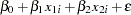
In this example, you test the simplest case to determine whether the model has constant returns to scale. Beginning with the general form of the Cobb-Douglas equation, take the natural log of both sides of the equation and define the regression equation.
 |
 |
 |
|||
 |
|
 |
|||
|
|
 |
|||
 |
|
 |
|||
 |
 |
|
|||
|
|
 |
|||
 |
|
 |
|||
 |
|
 |
|||
 |
|
 |
You are interested in determining whether the function exhibits constant returns to scale and test against the alternative that the returns are not constant. Hence,
|
 |
 |
|||
|
 |
 |
You can test this hypothesis using SAS by first creating the log variables, then using PROC REG to conduct an F test. Traditionally, you need to create both a full and a reduced model where the full model regresses  . The reduced model restates the hypothesis as
  and substitutes the new value for
  into the full model. Solving for the reduced model, you get the following:
 |
|
 |
|||
|
|
 |
|||
|
|
 |
|||
 |
|
 |
|||
 |
|
 |
Thus, you perform the simple linear regression  as the reduced model using the MODEL statement.
However, PROC REG can calculate the reduced model for you by using a TEST statement. After the full model is defined, the conditions for the F test are specified in the TEST statement and SAS automatically calculates the reduced model necessary to conduct the test. In this case, the conditions you use echo the hypothesis that the sum of the betas equals zero. Note that the variable names in the TEST statement correspond to the regressors and that each variable name represents its estimated coefficient.
   ** Create log variables **;
   data model (drop=_name_);
      set reg_data;
      y  = log(q);
      x1 = log(K);
      x2 = log(L);
   run;

   ** Run regression **;
   proc reg data=model;
      MODEL_1: model y = x1 x2;
      F_TEST: test x1+x2=1;
   run;
   quit;
The results are given in two separate tables, as shown in Figure 1.2 and Figure 1.3.
Figure 1.2 Fit Statistics and Parameter Estimates
| Analysis of Variance | |||||
|---|---|---|---|---|---|
| Source | DF | Sum of Squares |
Mean Square |
F Value | Pr > F |
| Model | 2 | 102.86112 | 51.43056 | 1152.36 | <.0001 |
| Error | 48 | 2.14227 | 0.04463 | ||
| Corrected Total | 50 | 105.00339 | |||
| Root MSE | 0.21126 | R-Square | 0.9796 |
|---|---|---|---|
| Dependent Mean | 23.60251 | Adj R-Sq | 0.9787 |
| Coeff Var | 0.89507 |
| Parameter Estimates | |||||
|---|---|---|---|---|---|
| Variable | DF | Parameter Estimate |
Standard Error |
t Value | Pr > |t| |
| Intercept | 1 | 2.46466 | 0.46928 | 5.25 | <.0001 |
| x1 | 1 | 0.66876 | 0.05930 | 11.28 | <.0001 |
| x2 | 1 | 0.36535 | 0.05535 | 6.60 | <.0001 |
Figure 1.3 F test Results
| Test F_TEST Results for Dependent Variable y | ||||
|---|---|---|---|---|
| Source | DF | Mean Square |
F Value | Pr > F |
| Numerator | 1 | 0.11003 | 2.47 | 0.1230 |
| Denominator | 48 | 0.04463 | ||
In the F test results, you find a  -value of
  . If the -value is less than the chosen significance level, then you reject the hypothesis in favor of the alternative. If the -value is greater than the chosen significance level, then there is insufficient evidence to reject the null hypothesis. If you assume a significance level of 0.05 for this example, then
  , and you fail to reject the hypothesis. You find that the model demonstrates constant returns to scale.
Conducting a t test for Non-Constant Returns to Scale
If you want to perform a specific test for either increasing or decreasing returns to scale, then you need to use a one-sided t test. In the case of increasing returns, you test the following hypothesis and alternative:
|
|
|
|||
|
|
 |
The case of decreasing returns works similarly. You test the following hypothesis and alternative:
|
|
|
|||
|
|
 |
You use the same MODEL statement that you used in the preceding F test to conduct this t test for increasing returns to scale. However, you also ask PROC REG to return a covariance matrix by specifying the COVB option on the MODEL statement. This enables you to compute the standard error of a linear combination of parameter estimates. The necessary code and its results follow in Figure 1.4:
   ** t Test Regression **;
   proc reg data=model;
      T_TEST: model y = x1 x2 / covb;
   run;
   quit;
Figure 1.4 Model Results and Covariance Matrix
| Analysis of Variance | |||||
|---|---|---|---|---|---|
| Source | DF | Sum of Squares |
Mean Square |
F Value | Pr > F |
| Model | 2 | 102.86112 | 51.43056 | 1152.36 | <.0001 |
| Error | 48 | 2.14227 | 0.04463 | ||
| Corrected Total | 50 | 105.00339 | |||
| Root MSE | 0.21126 | R-Square | 0.9796 |
|---|---|---|---|
| Dependent Mean | 23.60251 | Adj R-Sq | 0.9787 |
| Coeff Var | 0.89507 |
| Parameter Estimates | |||||
|---|---|---|---|---|---|
| Variable | DF | Parameter Estimate |
Standard Error |
t Value | Pr > |t| |
| Intercept | 1 | 2.46466 | 0.46928 | 5.25 | <.0001 |
| x1 | 1 | 0.66876 | 0.05930 | 11.28 | <.0001 |
| x2 | 1 | 0.36535 | 0.05535 | 6.60 | <.0001 |
| Covariance of Estimates | |||
|---|---|---|---|
| Variable | Intercept | x1 | x2 |
| Intercept | 0.2202250596 | -0.015334657 | 0.0054015337 |
| x1 | -0.015334657 | 0.0035162514 | -0.003054157 |
| x2 | 0.0054015337 | -0.003054157 | 0.0030639604 |
You construct the t statistic using the results such that
 |
|
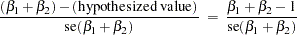 |
You construct the t statistic using the results such that
|
|
|
where the standard error (se) of the parameter estimates,  , is computed as
 |
|
 |
by using the results in the covariance matrix.
You can either compute the t statistic by hand, using the results in the ANOVA table and the preceding equation, or you can use an OUTEST statement in PROC REG to achieve the same result. The following code demonstrates how to use the OUTEST statement and its results in Figure 1.5.
   ** t Test Regression with OUTEST statement **;
   proc reg data=model outest=est covout edf;
      T_TEST_OUT: model y = x1 x2 / covb;
   run;
   quit;
   ** Calculate t statistic**;
   ** Keep the parameter estimates, error degrees of freedom, **;
   ** variances, and covariance                               **;
   data parms;
      set est (where=(_type_='PARMS'));
      keep x1 x2 _edf_;
   run;
   data varx1;
      set est (where=(_name_='x1'));
      varx1=x1;
      covx1x2=x2;
      keep varx1 covx1x2;
   run;
   data varx2;
      set est (where=(_name_='x2'));
      varx2=x2;
      keep varx2;
   run;
   ** Calculate the standard error for the denominator, **;
   ** the t statistic, and the p-values                 **;
   data ttest;
      merge parms varx1 varx2;
      se_x1x2 = sqrt(varx1 + varx2 + (2*covx1x2));
      t = (x1 + x2 - 1)/se_x1x2;
      p_inc = 1 - probt(t,_edf_);
      p_dec = probt(t,_edf_);
   run;
      ** Print and view the results **;
    proc print data=ttest;
       var t _edf_ p_inc p_dec;
       title "t statistic and p-values for model";
    run;
Figure 1.5 Model Results
| t statistic and p-values for model |
| Obs | t | _EDF_ | p_inc | p_dec |
|---|---|---|---|---|
| 1 | 1.57014 | 48 | 0.061476 | 0.93852 |
As with the F test, you compare the -values with your chosen level of significance. Assuming a significance level of 0.05, you compare the -value for increasing returns to scale. If the -value is greater than the chosen significance level, then there is insufficient evidence to reject the null hypothesis. Since  , you fail to reject the hypothesis. Similarly, you compare the -value for decreasing returns to scale to your chosen level of significance. Since
  , you fail to reject the hypothesis. The model is clearly demonstrating constant returns to scale.
References
-
Mendenhall, William and Terry Sincich (2003), A Second Course in Statistics: Regression Analysis, Sixth Edition, New Jersey: Pearson Education Inc.
-
Nicholson, W. (1992), Microeconomic Theory: Basic Principles and Extensions, Fifth Edition, Fort Worth: Dryden Press.
-
U.S. Census Bureau (2003), "Annual Survey of Manufactures, 2001 Geographic Area Statistics," http://www.census.gov/mcd/asm-as3.html.
-
Wooldridge, Jeffrey M. (2003), Introductory Econometrics: A Modern Approach, Second Edition, Ohio: South-Western.
-
Zellner, Arnold (1971), An Introduction to Bayesian Inference in Econometrics, New York: Wiley.
These sample files and code examples are provided by SAS Institute Inc. "as is" without warranty of any kind, either express or implied, including but not limited to the implied warranties of merchantability and fitness for a particular purpose. Recipients acknowledge and agree that SAS Institute shall not be liable for any damages whatsoever arising out of their use of this material. In addition, SAS Institute will provide no support for the materials contained herein.
ata census_data;
   input state $ type $ am;
   datalines;
AL q 28762420000
AL K 2818886000
AL L 544806000
AK q 1153433000
AK K 97292000
AK L 18942000
AZ q 27900974000
AZ K 2593261000
AZ L 245413000
AR q 19392561000
AR K 1410061000
AR L 367624000
CA q 196182882000
CA K 19628560000
CA L 2296334000
CO q 20609367000
CO K 2083882000
CO L 224728000
CT q 27298479000
CT K 1783242000
CT L 315068000
DE q 5209618000
DE K 352875000
DE L 59829000
DC q 170633000
DC K 22435000
DC L 3714000
FL q 39767726000
FL K 2506475000
FL L 555402000
GA q 55426485000
GA K 3408828000
GA L 826574000
HI q 1261303000
HI K 157221000
HI L 18343000
ID q 6383900000
ID K 1157786000
ID L 9069000
IL q 95342475000
IL K 6357175000
IL L 1278831000
IN q 67173341000
IN K 5272833000
IN L 978646000
IO q 28615467000
IO K 1804159000
IO L 356074000
KS q 18987474000
KS K 1178162000
KS L 280314000
KY q 39062786000
KY K 3499977000
KY L 455748000
LA q 27463050000
LA K 3259885000
LA L 256824000
ME q 6698567000
ME K 755909000
ME L 120642000
MD q 18705455000
MD K 1333239000
MD L 218330000
MA q 45132888000
MA K 3615304000
MA L 520200000
MI q 93366860000
MI K 6981199000
MI L 1299481000
MN q 36567010000
MN K 2579422000
MN L 513688000
MS q 17184299000
MS K 1169221000
MS L 360610000
MO q 43071878000
MO K 2834926000
MO L 526652000
MT q 1876897000
MT K 191380000
MT L 27386000
NB q 10460265000
NB K 697928000
NB L 172999000
NV q 3260969000
NV K 249037000
NV L 51573000
NH q 11129674000
NH K 854626000
NH L 134236000
NJ q 49432983000
NJ K 3644389000
NJ L 555738000
NM q 13487517000
NM K 630512000
NM L 56972000
NY q 75858926000
NY K 5074888000
NY L 1049318000
NC q 79790807000
NC K 5207500000
NC L 1192012000
ND q 2008799000
ND K 233693000
ND L 31447000
OH q 112361392000
OH K 7364383000
OH L 1494596000
OK q 17226649000
OK K 1495963000
OK L 241863000
OR q 25100453000
OR K 2899991000
OR L 314114000
PA q 86116509000
PA K 6024692000
PA L 1187997000
RI q 5462493000
RI K 350655000
RI L 103787000
SC q 33343682000
SC K 2769701000
SC L 536612000
SD q 4352357000
SD K 194857000
SD L 64773000
TN q 44527758000
TN K 4620591000
TN L 741421000
TX q 127579894000
TX K 11247496000
TX L 1340712000
UT q 11689959000
UT K 1281331000
UT L 169255000
VT q 4028276000
VT K 714803000
VT L 57719000
VA q 43180687000
VA K 2702950000
VA L 549218000
WA q 31534413000
WA K 2173424000
WA L 424129000
WV q 8980535000
WV K 570564000
WV L 112022000
WI q 54974219000
WI K 3710392000
WI L 829277000
WY q 1030583000
WY K 83569000
WY L 12209000
;
run;


** Manipulate the data for running regression and for plotting data **;
proc sort data=census_data;
   by state;
run;

** reg_data is the data set you use for running the regression **;
proc transpose data=census_data out=reg_data
   (rename = (Col1=q Col2=K Col3=L));
   var am;
   by state;
run;

data newdata;
   set census_data;
   lnam=log(am);
   if type='q' then do;
      format lnam dollar15.2;
      end;
   else if type='K' then do;
      format lnam dollar15.2;
      end;
   else if type='L' then do;
      delete;
      end;
run;
** plot_data is the data set you use for plotting the data **;
data plot_data;
   merge newdata (in=a) reg_data (in=b);
   by state;
   if a and b;
   lnl=round(log(L),.01);
   keep state type lnam lnl;
run;

** Create graph **;
proc gplot data=plot_data;
   plot lnam*state=type / nolegend haxis=axis1 vaxis=axis2;
   plot2 lnl*state / vaxis=axis3;
   symbol1 c=blue  i=join v=star;
   symbol2 c=green i=join v=dot;
   symbol3 c=red   i=join v=plus ;
   axis1 label=('State');
   axis2 label=(angle=90 'Value Added, Capital (in log dollars)')
      order=(0 to 30 by 5);
   axis3 label=(angle=90 'Labor (in log hours)')
      order=(0 to 30 by 5);
   title "1997 Production by State";
   footnote1 c=blue  '     *  Capital'
             c=red   '     +  Labor'
             c=green '     .  Value Added';
   footnote2 j=l 'Source: U.S. Census Bureau, Annual Survey of Manufactures,';
   footnote3 j=l '        2001 Geographic Area Statistics';
run;
quit;
title; footnote;

** Create log variables **;
data model (drop=_name_);
   set reg_data;
   y  = log(q);
   x1 = log(K);
   x2 = log(L);
run;

** Run regression **;
proc reg data=model;
   MODEL_1: model y = x1 x2;
   F_TEST: test x1+x2=1;
run;
quit;

** t Test Regression **;
proc reg data=model;
   T_TEST: model y = x1 x2 / covb;
run;
quit;

** t Test Regression with OUTEST statement **;
proc reg data=model outest=est covout edf;
   T_TEST_OUT: model y = x1 x2 / covb;
run;
quit;
** Calculate t statistic**;
** Keep the parameter estimates, error degrees of freedom, **;
** variances, and covariance                               **;
data parms;
   set est (where=(_type_='PARMS'));
   keep x1 x2 _edf_;
run;
data varx1;
   set est (where=(_name_='x1'));
   varx1=x1;
   covx1x2=x2;
   keep varx1 covx1x2;
run;
data varx2;
   set est (where=(_name_='x2'));
   varx2=x2;
   keep varx2;
run;
** Calculate the standard error for the denominator, **;
** the t statistic, and the p-values                 **;
data ttest;
   merge parms varx1 varx2;
   se_x1x2 = sqrt(varx1 + varx2 + (2*covx1x2));
   t = (x1 + x2 - 1)/se_x1x2;
   p_inc = 1 - probt(t,_edf_);
   p_dec = probt(t,_edf_);
run;
** Print and view the results **;
 proc print data=ttest;
    var t _edf_ p_inc p_dec;
    title "t statistic and p-values for model";
 run;
These sample files and code examples are provided by SAS Institute Inc. "as is" without warranty of any kind, either express or implied, including but not limited to the implied warranties of merchantability and fitness for a particular purpose. Recipients acknowledge and agree that SAS Institute shall not be liable for any damages whatsoever arising out of their use of this material. In addition, SAS Institute will provide no support for the materials contained herein.
| Type: | Sample |
| Date Modified: | 2017-08-01 12:43:45 |
| Date Created: | 2017-08-01 10:03:56 |
Operating System and Release Information
| Product Family | Product | Host | SAS Release | |
| Starting | Ending | |||
| SAS System | SAS/ETS | z/OS | ||
| z/OS 64-bit | ||||
| OpenVMS VAX | ||||
| Microsoft® Windows® for 64-Bit Itanium-based Systems | ||||
| Microsoft Windows Server 2003 Datacenter 64-bit Edition | ||||
| Microsoft Windows Server 2003 Enterprise 64-bit Edition | ||||
| Microsoft Windows XP 64-bit Edition | ||||
| Microsoft® Windows® for x64 | ||||
| OS/2 | ||||
| Microsoft Windows 8 Enterprise 32-bit | ||||
| Microsoft Windows 8 Enterprise x64 | ||||
| Microsoft Windows 8 Pro 32-bit | ||||
| Microsoft Windows 8 Pro x64 | ||||
| Microsoft Windows 8.1 Enterprise 32-bit | ||||
| Microsoft Windows 8.1 Enterprise x64 | ||||
| Microsoft Windows 8.1 Pro 32-bit | ||||
| Microsoft Windows 8.1 Pro x64 | ||||
| Microsoft Windows 10 | ||||
| Microsoft Windows 95/98 | ||||
| Microsoft Windows 2000 Advanced Server | ||||
| Microsoft Windows 2000 Datacenter Server | ||||
| Microsoft Windows 2000 Server | ||||
| Microsoft Windows 2000 Professional | ||||
| Microsoft Windows NT Workstation | ||||
| Microsoft Windows Server 2003 Datacenter Edition | ||||
| Microsoft Windows Server 2003 Enterprise Edition | ||||
| Microsoft Windows Server 2003 Standard Edition | ||||
| Microsoft Windows Server 2003 for x64 | ||||
| Microsoft Windows Server 2008 | ||||
| Microsoft Windows Server 2008 R2 | ||||
| Microsoft Windows Server 2008 for x64 | ||||
| Microsoft Windows Server 2012 Datacenter | ||||
| Microsoft Windows Server 2012 R2 Datacenter | ||||
| Microsoft Windows Server 2012 R2 Std | ||||
| Microsoft Windows Server 2012 Std | ||||
| Microsoft Windows XP Professional | ||||
| Windows 7 Enterprise 32 bit | ||||
| Windows 7 Enterprise x64 | ||||
| Windows 7 Home Premium 32 bit | ||||
| Windows 7 Home Premium x64 | ||||
| Windows 7 Professional 32 bit | ||||
| Windows 7 Professional x64 | ||||
| Windows 7 Ultimate 32 bit | ||||
| Windows 7 Ultimate x64 | ||||
| Windows Millennium Edition (Me) | ||||
| Windows Vista | ||||
| Windows Vista for x64 | ||||
| 64-bit Enabled AIX | ||||
| 64-bit Enabled HP-UX | ||||
| 64-bit Enabled Solaris | ||||
| ABI+ for Intel Architecture | ||||
| AIX | ||||
| HP-UX | ||||
| HP-UX IPF | ||||
| IRIX | ||||
| Linux | ||||
| Linux for x64 | ||||
| Linux on Itanium | ||||
| OpenVMS Alpha | ||||
| OpenVMS on HP Integrity | ||||
| Solaris | ||||
| Solaris for x64 | ||||
| Tru64 UNIX | ||||