Sample 60852: A Specification Test for Non-Nested Regression Models
 |  |  |  |  |
Overview
 |
In econometrics, researchers are constantly faced with the fundamental problem of choosing between models. The seminal contributions of Cox (1961) to the testing of separate families of hypotheses and Pesaran (1974) to the testing of non-nested linear regressions have lead to a burgeoning literature on the testing for non-nested models. As McAleer (1995) points out, prior to 1982, there were only about 15 published papers testing non-nested regression models. Over the last decade, however, more than 100 papers have been published.
Consider the following two models (refer to Pesaran and Deaton 1978):
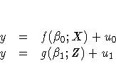
where y is an (nT)x1 vector of observations on all the n dependent variables, f(·) and g(·) are the corresponding vectors of predictions, u0 and u1, of errors, and X and Z are matrices of predetermined variables. As seen above, f(·) is not nested within g(·) and vice versa. A solution consists in nesting f(·) within more general models in which the variables Z appear explicitly as exogenous or endogenous variables.
One particular way of choosing between the two hypotheses is the J-test, suggested by Davidson and Mackinnon (1981). Estimate the comprehensive model
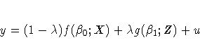
note that  is refered to as the mixing parameter hereafter). When no a priori information is available, the mixing parameter is not identifiable in the comprehensive model. The J-test works around this by replacing g(·) with the fitted values from a regression of y on Z and testing the mixing parameter for statistical significance.
This example illustrates a way to test the specification of a consumption function. The extension of this example to other non-nested models and multiple hypotheses is straightforward.
Analysis
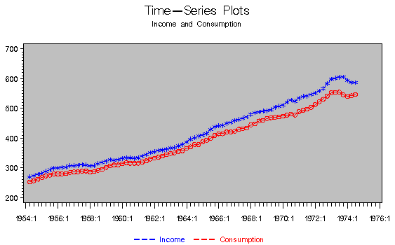
This example illustrates a specification problem in analyzing the relationship between consumption and income using U.S. quarterly data. One simple model postulates a linear relationship between consumption, income, and wealth; the influence of lagged income operates through the wealth term. Denoting consumption by c, income by y, and wealth by w, you postulate
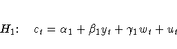
where ut denotes a normally distributed disturbance vector.
An alternative is to estimate an equation containing lagged consumption as an explanatory variable. This can be thought of as a variant of Duesenberry's (1949) relative income hypothesis. The model can be postulated as
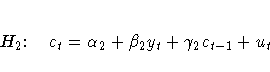
As seen above, the H1 and H2 models are non-nested.
The comprehensive models
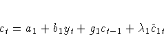
and
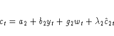
where  and
and  are the coefficients of the fitted values under H1 and H2, respectively, are both estimated. The J-test is applied by testing the mixing parameter, , for significance in each model.
The data set consists of seasonally adjusted quarterly time series of real 1958 prices, consumers' expenditure on non-durable goods and personal disposable income. These were collected from the Survey of Current Business and are used by Pesaran and Deaton (1978).
   data spec;
      input yr qr c y w;
      c_lag=lag(c);
      date = yyq( yr, qr );
      format date yyqc.;
      datalines;
   1954 2  253  270  0
   1954 3  257  274  17
   1954 4  262  279  34
   1955 1  268  282  51
   ...
   ;
   run;
Before the J-test can be performed, the fitted values from the two models must be calculated. The AUTOREG procedure can fit several different regressions with the inclusion of multiple model statements. In this example, two model statements are used, corresponding to the two hypotheses. For each MODEL statement an output data set is created with the OUT= option. These data sets contain the predicted values CHAT1 and CHAT2, as specified by the P= option. The DATA step merges the original data set with the two predicted data sets for use in the J-test.
    proc autoreg data=spec ;
       model c = y w;              /* model for H1 */
       output out=model1 p=chat1;
       model c = y c_lag;          /* model for H2 */
       output out=model2 p=chat2;
    run;

    data spec2;
       set spec ;
       set model1;
       set model2;
Because of the limits of the J-test, it is often wise to test twice for the significance of the mixing parameter by reversing the roles of the hypotheses. The AUTOREG procedure estimates the two comprehensive models. The coefficients of CHAT1 and CHAT2 correspond to a test of the significance of the mixing parameter, . To reject a model requires that the mixing parameter be insignificantly different from 0.
    proc autoreg data=spec2;
       model c = y c_lag chat1;
       model c = y w chat2;
    run;
The first comprehensive model yields the following parameter estimates:
|
|
The estimate for is 1.0185 with a p-value of 0.0001. As it is highly significant and statistically indistinguishable from 1, it provides further support to the previous conclusion that H1 should be rejected in favor of H2.
References
Cox, D.R. (1961), ``Tests of Separate Families of Hypotheses," Proceedings of the Fourth Berkeley Symposium on Mathematical Statistics and Probability, 1, Berkeley: University of California Press.
Davidson and Mackinnon (1981), ``Several Tests for Model Specification in the Presence of Alternative Hypotheses," Econometrica, 49, 781-793.
Duesenberry, J.S. (1949), Income, Saving, and the Theory of Consumer Behavior, Cambridge, MA: Harvard University Press.
Greene, W.H. (1993), Econometric Analysis, Second Edition, New York: Macmillan Publishing Company.
McAleer M. (1995), ``The Significance of Testing Empirical Non-nested Models," Journal of Econometrics, 67, 150-171.
Pesaran, M.H. (1974), ``On the General Problem of Model Selection," Review of Economic Studies, 41, 153-171.
Pesaran, M.H. and Deaton, A.S. (1978), ``Testing Non-nested Nonlinear Regression Models," Econometrica, 46, 677-694.
SAS Institute Inc. (1993), SAS/ETS Users's Guide, Version 6, Second Edition, Cary, NC: SAS Institute Inc.
Stone, J.R.E. (1973), ``Personal Spending and Saving in Post-War Britain," in Economic Structure and Development: Essays in Honour of Jan Tinbergen, eds. H.C. Bos, H. Linnemann, and P. De Wolff, Amsterdam: North Holland, 79-98.
These sample files and code examples are provided by SAS Institute Inc. "as is" without warranty of any kind, either express or implied, including but not limited to the implied warranties of merchantability and fitness for a particular purpose. Recipients acknowledge and agree that SAS Institute shall not be liable for any damages whatsoever arising out of their use of this material. In addition, SAS Institute will provide no support for the materials contained herein.
/* A Specification Test for Non-Nested Models */

 data spec;
   input yr qr c y w;
     c_lag=lag(c);
     date = yyq( yr, qr );
     format date yyqc.;
 datalines;
1954 2  253  270  0
1954 3  257  274  17
1954 4  262  279  34
1955 1  268  282  51
1955 2  273  289  66
1955 3  276  294  82
1955 4  280  299  100
1956 1  280  300  118
1956 2  280  302  138
1956 3  281  303  160
1956 4  285  308  182
1957 1  287  308  205
1957 2  287  309  226
1957 3  289  311  249
1957 4  290  310  271
1958 1  286  307  291
1958 2  288  308  312
1958 3  292  315  333
1958 4  295  319  356
1959 1  302  323  380
1959 2  307  328  401
1959 3  310  326  422
1959 4  310  328  437
1960 1  314  332  455
1960 2  318  334  473
1960 3  316  334  489
1960 4  316  332  507
1961 1  316  334  522
1961 2  320  340  540
1961 3  324  345  559
1961 4  330  352  581
1962 1  333  355  603
1962 2  336  359  624
1962 3  340  360  647
1962 4  345  363  667
1963 1  349  367  685
1963 2  351  369  703
1963 3  356  374  721
1963 4  358  379  739
1964 1  366  387  760
1964 2  371  397  781
1964 3  379  402  807
1964 4  379  407  830
1965 1  388  411  858
1965 2  393  416  881
1965 3  400  430  904
1965 4  409  438  933
1966 1  415  442  962
1966 2  415  443  989
1966 3  421  450  1017
1966 4  421  454  1045
1967 1  424  459  1079
1967 2  430  463  1114
1967 3  432  468  1147
1967 4  434  472  1183
1968 1  445  480  1220
1968 2  448  486  1255
1968 3  458  488  1293
1968 4  460  491  1323
1969 1  466  492  1354
1969 2  469  496  1381
1969 3  470  504  1408
1969 4  472  508  1442
1970 1  474  511  1478
1970 2  478  522  1514
1970 3  481  528  1559
1970 4  478  524  1605
1971 1  490  535  1652
1971 2  494  541  1697
1971 3  498  542  1744
1971 4  504  547  1789
1972 1  513  552  1832
1972 2  523  559  1871
1972 3  531  567  1906
1972 4  542  584  1942
1973 1  553  599  1984
1973 2  554  602  2030
1973 3  555  605  2078
1973 4  546  606  2128
1974 1  540  594  2187
1974 2  543  587  2242
1974 3  547  587  2286
;
run;

proc autoreg data=spec ;
   model c = y w;
   output out=model1 p=chat1;
   model c = y c_lag;
   output out=model2 p=chat2;
run;

data spec2;
   set spec ;
   set model1;
   set model2;
run;

proc autoreg data=spec2;
   model c = y c_lag chat1;
   model c = y w chat2;
run;
quit;

proc gplot data=spec;
   plot y*date c*date / overlay cframe=ligr
                        haxis=axis1 vaxis=axis2;
   title 'Time-Series Plots';
   title2 'Income and Consumption';
   footnote1 c=blue ' --- Income'
             c=red  '  --- Consumption';
   symbol1 c=blue i=join v=star;
   symbol2 c=red  i=join v=circle;
   axis1 label=none;
   axis2 label=none;
run;
quit;
These sample files and code examples are provided by SAS Institute Inc. "as is" without warranty of any kind, either express or implied, including but not limited to the implied warranties of merchantability and fitness for a particular purpose. Recipients acknowledge and agree that SAS Institute shall not be liable for any damages whatsoever arising out of their use of this material. In addition, SAS Institute will provide no support for the materials contained herein.
| Type: | Sample |
| Date Modified: | 2017-08-01 09:58:54 |
| Date Created: | 2017-07-31 15:26:48 |
Operating System and Release Information
| Product Family | Product | Host | SAS Release | |
| Starting | Ending | |||
| SAS System | SAS/ETS | z/OS | ||
| z/OS 64-bit | ||||
| OpenVMS VAX | ||||
| Microsoft® Windows® for 64-Bit Itanium-based Systems | ||||
| Microsoft Windows Server 2003 Datacenter 64-bit Edition | ||||
| Microsoft Windows Server 2003 Enterprise 64-bit Edition | ||||
| Microsoft Windows XP 64-bit Edition | ||||
| Microsoft® Windows® for x64 | ||||
| OS/2 | ||||
| Microsoft Windows 8 Enterprise 32-bit | ||||
| Microsoft Windows 8 Enterprise x64 | ||||
| Microsoft Windows 8 Pro 32-bit | ||||
| Microsoft Windows 8 Pro x64 | ||||
| Microsoft Windows 8.1 Enterprise 32-bit | ||||
| Microsoft Windows 8.1 Enterprise x64 | ||||
| Microsoft Windows 8.1 Pro 32-bit | ||||
| Microsoft Windows 8.1 Pro x64 | ||||
| Microsoft Windows 10 | ||||
| Microsoft Windows 95/98 | ||||
| Microsoft Windows 2000 Advanced Server | ||||
| Microsoft Windows 2000 Datacenter Server | ||||
| Microsoft Windows 2000 Server | ||||
| Microsoft Windows 2000 Professional | ||||
| Microsoft Windows NT Workstation | ||||
| Microsoft Windows Server 2003 Datacenter Edition | ||||
| Microsoft Windows Server 2003 Enterprise Edition | ||||
| Microsoft Windows Server 2003 Standard Edition | ||||
| Microsoft Windows Server 2003 for x64 | ||||
| Microsoft Windows Server 2008 | ||||
| Microsoft Windows Server 2008 R2 | ||||
| Microsoft Windows Server 2008 for x64 | ||||
| Microsoft Windows Server 2012 Datacenter | ||||
| Microsoft Windows Server 2012 R2 Datacenter | ||||
| Microsoft Windows Server 2012 R2 Std | ||||
| Microsoft Windows Server 2012 Std | ||||
| Microsoft Windows XP Professional | ||||
| Windows 7 Enterprise 32 bit | ||||
| Windows 7 Enterprise x64 | ||||
| Windows 7 Home Premium 32 bit | ||||
| Windows 7 Home Premium x64 | ||||
| Windows 7 Professional 32 bit | ||||
| Windows 7 Professional x64 | ||||
| Windows 7 Ultimate 32 bit | ||||
| Windows 7 Ultimate x64 | ||||
| Windows Millennium Edition (Me) | ||||
| Windows Vista | ||||
| Windows Vista for x64 | ||||
| 64-bit Enabled AIX | ||||
| 64-bit Enabled HP-UX | ||||
| 64-bit Enabled Solaris | ||||
| ABI+ for Intel Architecture | ||||
| AIX | ||||
| HP-UX | ||||
| HP-UX IPF | ||||
| IRIX | ||||
| Linux | ||||
| Linux for x64 | ||||
| Linux on Itanium | ||||
| OpenVMS Alpha | ||||
| OpenVMS on HP Integrity | ||||
| Solaris | ||||
| Solaris for x64 | ||||
| Tru64 UNIX | ||||