Sample 60816: Fitting a Capital Asset Pricing Model

Overview

The Capital Asset Pricing Model (CAPM) is one of the most common methods of relating the sensitivity of an individual company's stock return to the return of the market as a whole. Specifically, the CAPM linear relationship can be written as

$r_j - r_f=\frac{\sigma_j}{\sigma_m}(r_m - r_f)$

where r_j, r_f, and r_m are returns to security j, the risk-free asset and the market return, respectively. The term $\sigma_j/\sigma_m$ is the ratio of the standard deviations of returns on security j to the market.

A full development of the CAPM can be found in any introductory finance textbook (for example, Brealey and Myers 1988), and so is omitted here. There are, however, several econometric issues involved in the more general model

$r_j - r_f=\alpha_j + \beta_j(r_m - r_f) + \epsilon_j$

where $\alpha_j$ is an intercept term, and $\epsilon_j$ is an IID stochastic disturbance term with mean zero and variance $\sigma^2$ .

Two straightforward tests of this model are

a test of the null $\alpha_j=0$ against the alternative that it is not equal to 0. A rejection would cast some doubt on the theoretical model as $\alpha_j$ is assumed to be 0 in the first equation.
a test of the null $\beta_j=1$ against the alternative that it is not equal to 1. Failure to reject would imply that the movement of asset prices of a particular company is the same as that of the market as a whole.

This example uses stock returns from the Tandy Corporation to estimate a CAPM and perform some general tests of the model.

Analysis

The CAPM relates the sensitivity of an individual company's stock returns to the returns of the market as a whole. Estimating a model for a particular firm requires data on the market rate of return (typically a composite index such as the S&P 500 or the Dow Jones Industrial Average), the risk-free rate of return (usually a short-term Treasury bill), and stock returns from the company of interest.

The data for this example consist of monthly observations from January 1978 through December 1987 on the market return, the risk-free rate, and the return on the Tandy Corporation's common stock. Using a SAS DATA step, enter the data and create two new variables, R_TANDY = TANDY - R_F and R_MKT = R_M - R_F, that correspond to the risk premiums for the Tandy Corporation and the Market. A risk premium is the excess return of a security over the risk-free rate or, rather, the extra return that investors require for bearing risk.

   data tandy;
      input r_m r_f tandy @@;
      r_tandy = tandy - r_f;
      r_mkt = r_m -r_f;
      label r_m='Market Rate of Return'
            r_f='Risk-Free Rate of Return'
            tandy='Rate of Return for Tandy Corporation'
            r_tandy='Risk Premium for Tandy Corporation'
            r_mkt='Risk Premium for Market';
      datalines;
   -.045 .00487 -.075
    .063 .00491  .055
    .071 .00528  .194
     ... more data ...
   ;
   run;

It is always a good idea to look at the data to be sure that it was input as expected. A simple plot allows for a visual assessment of the appropriateness of the proposed model. The following code uses the GPLOT procedure to plot the risk premium of the Tandy Corporation against the risk premium of the Market.

   proc gplot data=tandy;
     plot r_tandy * r_mkt / haxis=axis1 hminor=4 cframe=ligr
                            vaxis=axis2 vminor=4;
     symbol1 c=blue v=star;
     axis1 order=(-0.3 to 0.2 by 0.1);
     axis2 label=(angle=90 'Tandy Corp. Risk Premium')
           order=(-0.4 to 0.6 by 0.2);
     title 'TANDY Corporation CAPM Example';
     title2'Plot of Risk Premiums';
     title3'Tandy Corporation versus the Market';
   run;

The plot of the Tandy data set above indicates that there is a positive relationship between the risk premium of the market and the risk premium of the Tandy Corporation's stock. This positive relationship seems sensible: as the market return increases, so should the return of most stocks. Based on this visual evidence, a linear model between R_TANDY and R_MKT is not unreasonable.

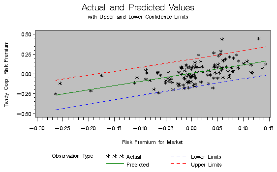
The AUTOREG procedure specifies a linear regression of R_TANDY on R_MKT. Note that a constant term is automatically included in the model unless the NOINT option is specified. The DWPROB option requests the Durbin-Watson test for autocorrelation of the residuals. The TEST statement enables you to perform hypothesis tests on parameter estimates; the following TEST statement is requesting a test that the coefficient of R_MKT is equal to 1. In addition, the OUTPUT data set TANDYOUT contains the predicted values of R_TANDY, the residuals of the regression, and the upper and lower bounds of the 90% confidence interval.

   proc autoreg data=tandy;
     model r_tandy = r_mkt / dwprob;
     test r_mkt = 1;
     output out=tandyout p=p r=r ucl=u lcl=l alphacli=.10;
     title2;
     title3;
   run;

The AUTOREG Procedure

Dependent Variable	r_tandy
	Risk Premium for Tandy Corporation

Ordinary Least Squares Estimates
SSE	1.31740165	DFE	118
MSE	0.01116	Root MSE	0.10566
SBC	-191.29942	AIC	-196.8744
Regress R-Square	0.3191	Total R-Square	0.3191
Durbin-Watson	1.9334	Pr < DW	0.3587
Pr > DW	0.6413

Variable	DF	Estimate	Standard Error	t Value	Approx Pr > \|t\|	Variable Label
Intercept	1	0.0107	0.009698	1.10	0.2740
r_mkt	1	1.0500	0.1412	7.44	<.0001	Risk Premium for Market

Test 1
Source	DF	Mean Square	F Value	Pr > F
Numerator	1	0.001400	0.13	0.7239
Denominator	118	0.011164

The output provides information about the appropriateness of the model chosen. The parameter estimate for $\alpha$ , the intercept, is not significantly different from 0. The estimate for $\beta$ , the coefficient of R_MKT, is 1.05 and is highly significant. So, not altogether unexpectedly, it seems that the market risk premium is a factor in the risk premium for the Tandy Corporation.

The F-statistic for the test that the coefficient of R_MKT is equal to one is 0.1254 with an associated p-value of 0.724, implying that there is little evidence that this coefficient is different from 1.0. Thus there is little evidence that the returns of the Tandy stock were any more or less volatile than the returns of the market.

R2 measures the proportion of the total variation of Y explained by the regression of Y on the independent variable, X. The R² value of 0.319 means that about 32% of the variation in the risk premium of Tandy Corporation stock can be explained by the risk premium of the market. Or, put another way, 68% of the risk premium of Tandy stock is firm specific.

The Durbin-Watson d statistic tests for autocorrelation and lack of independence of residuals, which is a common problem in time series data. The d statistic ranges from 0 to 4. A value close to 2.0 indicates that you cannot reject the null hypothesis of no autocorrelation. The calculated value of the d statistic in the CAPM for the Tandy Corporation is 1.933, and it has a p-value of 0.359. This value indicates that, for this model, you cannot reject the null hypothesis of independent (nonautocorrelated) residuals at typically chosen levels of significance.

Using PROC GPLOT, you can investigate the residuals for patterns that would indicate a violation of the underlying assumptions of the model.

   proc gplot data=tandyout;
     plot r * r_mkt / haxis=axis1 hminor=4 cframe=ligr
                      vaxis=axis2 vminor=4
                      vref=0.0;
     symbol1 c=green v=star;
     axis1 order=(-0.3 to 0.2 by 0.1);
     axis2 label=(angle=90 'Tandy Corp. Risk Premium')
           order=(-0.3 to 0.4 by 0.1);
     title 'TANDY Corporation CAPM Example';
     title2'OLS Residuals versus Market Risk Premium';
   run;

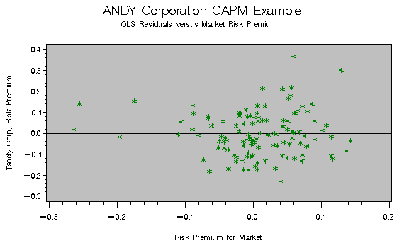This residual plot does not reveal any obvious patterns; the residuals appear randomly distributed about the reference line.

References

Berndt, Ernst R. (1991), The Practice of Econometrics: Classic and Contemporary, New York: Addison-Wesley.

Brealey, Richard A. and Myers, Stewart C. (1988), Principles of Corporate Finance, Third Edition, New York: McGraw-Hill.

SAS Institute Inc. (1993), SAS/ETS Software: Applications Guide 2, Version 6, First Edition: Econometric Modeling, Simulation, and Forecasting, Cary, NC: SAS Institute Inc., 15-30.

These sample files and code examples are provided by SAS Institute Inc. "as is" without warranty of any kind, either express or implied, including but not limited to the implied warranties of merchantability and fitness for a particular purpose. Recipients acknowledge and agree that SAS Institute shall not be liable for any damages whatsoever arising out of their use of this material. In addition, SAS Institute will provide no support for the materials contained herein.

/* Fitting a Capital Asset Pricing Model */

data tandy;
  input r_m r_f tandy @@;
  r_tandy = tandy - r_f;
  r_mkt = r_m -r_f;
  label r_m='Market Rate of Return'
        r_f='Risk-Free Rate of Return'
        tandy='Rate of Return for Tandy Corporation'
        r_tandy='Risk Premium for Tandy Corporation'
        r_mkt='Risk Premium for Market';
datalines;
-.045 .00487 -.075
 .063 .00491  .055
 .071 .00528  .194
-.189 .00685 -.206
 .058 .00761 -.046
 .026 .00764 -.094
-.013 .00728  .006
-.097 .00913 -.037
 .124 .00883  .032
 .080 .00753 -.038
 .065 .00602  .446
 .006 .00895 -.015
-.014 .01092 -.139
-.008 .01084  .092
-.033 .01154  .032
 .062 .01003  .241
-.079 .00949  .059
 .041 .00972  .053
-.006 .00714  .050
 .136 .00620  .454
 .065 .00646  .091
 .097 .00652  .084
-.017 .00714 -.123
-.082 .00678 -.058
-.029 .00712 -.190
-.003 .00741  .120
-.058 .00771  .029
-.035 .00688 -.096
 .097 .00606  .170
-.010 .00601 -.133
 .010 .00494 -.004
 .067 .00513  .176
 .079 .00607  .222
 .084 .00719  .086
 .011 .00761 -.135
 .014 .00772 -.148
 .095 .00789  .250
 .116 .00819  .170
 .112 .01073  .143
 .062 .00630  .256
 .025 .00731  .167
 .092 .01137  .212
-.009 .01096  .082
 .064 .01255  .136
-.031 .01169 -.063
 .069 .00816 -.037
-.101 .00946 -.101
 .003 .00908 -.163
 .122 .00503  .017
 .049 .00614  .273
 .028 .00599  .032
 .080 .00649 -.010
-.034 .00668 -.048
 .066 .00683  .082
-.030 .00672 -.100
-.058 .00627 -.231
 .146 .00852  .079
-.019 .00602  .027
 .012 .00586  .119
 .019 .00512  .091
 .050 .00526  .124
 .007 .00527 -.014
 .002 .00645 -.100
 .015 .00690  .085
 .123 .00769  .122
 .075 .00715  .096
 .039 .00802 -.005
 .086 .00747  .037
-.243 .01181 -.105
 .086 .00503  .041
 .015 .00860  .157
-.056 .00977  .022
 .067 .01025  .299
-.003 .01128 -.167
-.164 .01054 -.008
-.039 .00740 -.046
-.028 .01067 -.051
-.078 .00914  .023
 .008 .00563 -.026
 .014 .00648 -.042
 .043 .00686 -.004
 .048 .00673 -.168
 .000 .00702 -.083
-.012 .00693  .095
 .003 .00763 -.008
 .005 .00748 -.037
 .000 .00830 -.100
-.001 .00612  .005
 .008 .00650  .094
-.003 .00536  .087
 .012 .00562 -.119
 .026 .00577  .098
-.009 .00548 -.040
-.009 .00444 -.058
-.076 .00458 -.078
 .018 .00418  .242
 .148 .00454  .130
-.025 .00207 -.119
 .055 .00455  .087
-.260 .00358 -.246
 .005 .00545  .063
 .059 .00540  .021
 .049 .00523  .096
 .049 .00469  .094
 .049 .00343  .018
 .000 .00420  .094
 .065 .00437  .174
 .004 .00438 -.026
 .015 .00460  .027
-.070 .00288 -.190
-.055 .00571 -.011
 .013 .00479  .098
 .048 .00508 -.047
 .004 .00478 -.092
-.047 .00416 -.108
-.005 .00382 -.023
 .037 .00423 -.118
 .038 .00402  .045
-.015 .00520  .088
 .073 .00277  .040
;

proc gplot data=tandy;
  plot r_tandy * r_mkt / haxis=axis1 hminor=4 cframe=ligr
                         vaxis=axis2 vminor=4;
  symbol1 c=blue v=star;
  axis1 order=(-0.3 to 0.2 by 0.1);
  axis2 label=(angle=90 'Tandy Corp. Risk Premium')
        order=(-0.4 to 0.6 by 0.2);
  title 'TANDY Corporation CAPM Example';
  title2'Plot of Risk Premiums';
  title3'Tandy Corporation versus the Market';
run;


proc autoreg data=tandy;
  model r_tandy = r_mkt / dwprob;
  test r_mkt = 1;
  output out=tandyout p=p r=r ucl=u lcl=l alphacli=.10;
  title2;
  title3;
run;


proc gplot data=tandyout;
  plot r * r_mkt / haxis=axis1 hminor=4 cframe=ligr
                   vaxis=axis2 vminor=4
                   vref=0.0;
  symbol1 c=green v=star;
  axis1 order=(-0.3 to 0.2 by 0.1);
  axis2 label=(angle=90 'Tandy Corp. Risk Premium')
        order=(-0.3 to 0.4 by 0.1);
  title 'TANDY Corporation CAPM Example';
  title2'OLS Residuals versus Market Risk Premium';
run;


proc sort data=tandyout;
  by r_mkt;
run;

data regdata(keep=y_value pt_type r_mkt);
  set tandyout;
  label pt_type='Observation Type';
  array regvar{4} r_tandy p l u;
  array varlabel{4} $12 _temporary_
    ('Actual' 'Predicted' 'Lower Limits' 'Upper Limits');
  do i=1 to 4;
    y_value=regvar{i};
    pt_type=varlabel{i};
    output;
  end;
run;

proc gplot data=regdata;
  plot y_value*r_mkt=pt_type / haxis=axis1 hminor=4 cframe=ligr
                               vaxis=axis2 vminor=4;
  symbol1 c=black v=star;
  symbol2 c=blue i=join l=2;
  symbol3 c=green i=join l=1;
  symbol4 c=red i=join l=2;
  axis1 order=(-.3 to .15 by .05);
  axis2 label=(angle=90 'Tandy Corp. Risk Premium')
        order=(-.5 to .5 by .25);
  title1 "Actual and Predicted Values";
  title2 "with Upper and Lower Confidence Limits";
run;
quit;

These sample files and code examples are provided by SAS Institute Inc. "as is" without warranty of any kind, either express or implied, including but not limited to the implied warranties of merchantability and fitness for a particular purpose. Recipients acknowledge and agree that SAS Institute shall not be liable for any damages whatsoever arising out of their use of this material. In addition, SAS Institute will provide no support for the materials contained herein.

The Capital Asset Pricing Model (CAPM) is one of the most common methods of relating the sensitivity of an individual company's stock return to the return of the market as a whole.

Type:

Sample

Date Modified:	2017-07-25 14:51:59
Date Created:	2017-07-25 14:41:20

Operating System and Release Information

Product Family	Product	Host	SAS Release
Product Family	Product	Host	Starting	Ending
SAS System	SAS/ETS	z/OS
		z/OS 64-bit
		OpenVMS VAX
		Microsoft® Windows® for 64-Bit Itanium-based Systems
		Microsoft Windows Server 2003 Datacenter 64-bit Edition
		Microsoft Windows Server 2003 Enterprise 64-bit Edition
		Microsoft Windows XP 64-bit Edition
		Microsoft® Windows® for x64
		OS/2
		Microsoft Windows 8 Enterprise 32-bit
		Microsoft Windows 8 Enterprise x64
		Microsoft Windows 8 Pro 32-bit
		Microsoft Windows 8 Pro x64
		Microsoft Windows 8.1 Enterprise 32-bit
		Microsoft Windows 8.1 Enterprise x64
		Microsoft Windows 8.1 Pro 32-bit
		Microsoft Windows 8.1 Pro x64
		Microsoft Windows 10
		Microsoft Windows 95/98
		Microsoft Windows 2000 Advanced Server
		Microsoft Windows 2000 Datacenter Server
		Microsoft Windows 2000 Server
		Microsoft Windows 2000 Professional
		Microsoft Windows NT Workstation
		Microsoft Windows Server 2003 Datacenter Edition
		Microsoft Windows Server 2003 Enterprise Edition
		Microsoft Windows Server 2003 Standard Edition
		Microsoft Windows Server 2003 for x64
		Microsoft Windows Server 2008
		Microsoft Windows Server 2008 R2
		Microsoft Windows Server 2008 for x64
		Microsoft Windows Server 2012 Datacenter
		Microsoft Windows Server 2012 R2 Datacenter
		Microsoft Windows Server 2012 R2 Std
		Microsoft Windows Server 2012 Std
		Microsoft Windows XP Professional
		Windows 7 Enterprise 32 bit
		Windows 7 Enterprise x64
		Windows 7 Home Premium 32 bit
		Windows 7 Home Premium x64
		Windows 7 Professional 32 bit
		Windows 7 Professional x64
		Windows 7 Ultimate 32 bit
		Windows 7 Ultimate x64
		Windows Millennium Edition (Me)
		Windows Vista
		Windows Vista for x64
		64-bit Enabled AIX
		64-bit Enabled HP-UX
		64-bit Enabled Solaris
		ABI+ for Intel Architecture
		AIX
		HP-UX
		HP-UX IPF
		IRIX
		Linux
		Linux for x64
		Linux on Itanium
		OpenVMS Alpha
		OpenVMS on HP Integrity
		Solaris
		Solaris for x64
		Tru64 UNIX

Support

Sample 60816: Fitting a Capital Asset Pricing Model

Overview

Analysis

References

Operating System and Release Information