60782 - Estimating an Almost Ideal Demand System Model

Sample 60782: Estimating an Almost Ideal Demand System Model

Overview

The Almost Ideal Demand System (AIDS) model of Deaton and Muellbauer (1980b) has enjoyed great popularity in applied demand analysis. Starting from a specific cost function, the AIDS model gives the share equations in an n-good system as

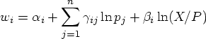
$w_i = \alpha_i + \sum_{j=1}^n { \gamma_{ij} \ln p_{j} } + \beta_i \ln (X/P)$

where w_i is the share associated with the ith good, $\alpha_i$ is the constant coefficient in the ith share equation, $\gamma_{ij}$ is the slope coefficient associated with the jth good in the ith share equation, p_j is the price on the jth good. X is the total expenditure on the system of goods given by

$X = \sum_{i=1}^n {p_{i} q_{i}}$

in which q_i is the quantity demanded for the ith good. P is the price index defined by

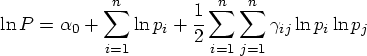
$\ln P = \alpha_0 + \sum_{i=1}^n { \ln p_i } + \frac{1}2 \sum_{i=1}^n \sum_{j=1}^n \gamma_{ij} \ln p_i \ln p_j$

in the nonlinear AIDS model. Deaton and Muellbauer (1980a) also suggested a linear approximation of the nonlinear AIDS model by specifying a linear price index given by

$\ln P = \sum_{i=1}^n {w_i \ln p_i}$

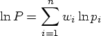
that gives rise to the linear approximate AIDS (LA-AIDS) model. In practice, the LA-AIDS model is more frequently estimated than the nonlinear AIDS model.

Conservation implies the following restrictions on the parameters in the nonlinear AIDS model:

$\sum_{i=1}^n \alpha_i = 1, \sum_{i=1}^n \beta_i = 0, \sum_{i=1}^n \gamma_{ij} = 0$

Homogeneity is satisfied if and only if, for all i

$\sum_{j=1}^n \gamma_{ij} = 0$

and symmetry is satisfied if

$\gamma_{ij} = \gamma_{ji}$

One advantage of the AIDS model is that the homogeneity and symmetry restrictions are easily imposed and tested.

Analysis

In this example, you can estimate a nonlinear AIDS model and LA-AIDS model using U.S. meat products data. The data consists of aggregate quarterly retail price and per capita consumption for four meat product categories including beef, pork, chicken, and turkey. The data period covers the first quarter of 1974 to the last quarter of 1999. The data were obtained from various USDA sources listed in the references. More detailed description of the data construction may be found in Piggott (1997).

To incorporate seasonality and trend in the U.S. meat consumption data, you augment the AIDS model with trigonometric variables and a time trend variable. Thus the share equations to be estimated are expressed as follows:

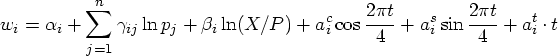
$w_i = \alpha_i + \sum_{j = 1}^n { \gamma_{ij} \ln {p_j}} + \beta_i \ln (X/P) + a^c_i \cos { \frac{2 \pi t}4 } + a^s_i \sin {\frac{2 \pi t}4} + a^t_i \cdot t$

where a^c_i and a^s_i represent parameters on the trigonometric variables, and a^t_i is the parameter on the time trend variable. Since the budget shares sum up to 1, these parameters should satisfy

$\sum_{i=1}^n{a^c_i} = 0, \sum_{i=1}^n{a^s_i} = 0, \sum_{i=1}^n{a^t_i}=0$

The following is a portion of the code used to create the data set. A second set of SAS statements is used to create the time trend variable and the seasonal variables. Total expenditures, X, and shares for each good are also computed.

   data aids_;
      input year qtr pop beef_q pork_q chick_q turkey_q beef_p pork_p chick_p
            turkey_p cpi pc_exp;
      date = yyq(year,qtr);
      format date yyq6.;


   ... more datalines ...

   ;
   run;

   data aids;
      set aids_;
      if year < 1975 then delete;
      t = _n_ ;
      co1 = cos(1/2*3.14159*t);
      co2 = cos(2/2*3.14159*t);

      si1 = sin(1/2*3.14159*t);
      si2 = sin(2/2*3.14159*t);

      x = beef_p*beef_q + pork_p*pork_q + chick_p*chick_q
          + turkey_p*turkey_q;

      w_beef = beef_p*beef_q/x;
      w_pork = pork_p*pork_q/x;
      w_chick = chick_p*chick_q/x;
      w_turkey = turkey_p*turkey_q/x;
   run;

The plot of the budget shares found in Figure 1.

   proc gplot data=aids;
      plot w_beef*date w_pork*date w_chick*date w_turkey*date/
           overlay cframe=ligr haxis=axis1 vaxis=axis2;
      title 'Budget Shares Plots';
      footnote1 c=blue '  *     beef   '
                c=red  '  .     pork  '
                c=green '  o    chicken  '
                c=black '  +    turkey   ';
      symbol1 c=blue i=join v=star;
      symbol2 c=red  i=join v=dot;
      symbol3 c=green i = join v = circle ;
      symbol4 c=black i = join v = plus ;
      axis1  label=('Time') ;
      axis2  label=(angle=90 'Budget Share');
   run;
   quit;

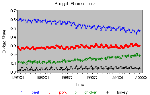Figure 1: Budget Shares Plots

Price and quantity variables in the data set are labeled in an obvious manner. Three variable names in the DATA step require some explanation. The variable named pop contains the U.S. population, cpi contains the consumer price index for all goods, and pc_exp is the per capita nominal personal consumption expenditures on all goods.

To obtain mean-scaled price data, you use the MEANS procedure. The means of each of the price variables are written to the OUT= data set as the b_m, p_m, c_m, and t_m variables. The original price variables are then divided by the mean variables in a subsequent DATA step.

   data aids ;
      if _n_ = 1 then set pm ;
      set aids ;

      pb_ = (beef_p/b_m);
      pp_ = (pork_p/p_m);
      pc_ = (chick_p/c_m);
      pt_ = (turkey_p/t_m);

      lpb = log(pb_);
      lpp = log(pp_);
      lpc = log(pc_);
      lpt = log(pt_);

      lx = log(x);

   /* Specify the linear price index for the LA-AIDS model */
      lp0 = sum(w_beef*lpb + w_pork*lpp + w_chick*lpc + w_turkey*lpt);
      lxp = lx-lp0;
   run;

The LA-AIDS model is estimated using the SYSLIN procedure. The ITSUR option specifies the iterated seemingly unrelated regression as the estimation method. The equations to be fit are then specified. Since budget shares sum to 1 in the system, one of the share equations is deleted to deal with the singularity problem. In this example, you eliminate the share equation for turkey. Whichever one is eliminated should not have any effect on the results. The parameters associated with the share equation that is deleted can be recovered through the parameter restrictions implied by the homogeneity, symmetry, and conservation properties. The parameter restrictions can be imposed through the SRESTRICT statement.

   proc syslin itsur data = aids outest = fin1;
      b: model w_beef = lpb lpp lpc lpt lxp co1 si1 t ;
      p: model w_pork = lpb lpp lpc lpt lxp co1 si1 t ;
      c: model w_chick = lpb lpp lpc lpt lxp co1 si1 t ;

      srestrict
      /*symmetry restrictions */
      b.lpp = p.lpb ,
      b.lpc = c.lpb ,
      p.lpc = c.lpp ,
      /* homogeneity restrictions*/
      b.lpb + b.lpp + b.lpc + b.lpt = 0 ,
      p.lpb + p.lpp + p.lpc + p.lpt = 0 ,
      c.lpb + c.lpp + c.lpc + c.lpt = 0;
   run;

The parameter estimates in the beef equation are given in Figure 2.

Parameter Estimates - Beef

Variable	DF	Estimate	StdErr	tValue	Probt
Intercept	1	0.397899	0.400708	0.99	0.3234
lpb	1	0.041175	0.012686	3.25	0.0016
lpp	1	-0.00407	0.008127	-0.50	0.6181
lpc	1	-0.04926	0.00541	-9.10	<.0001
lpt	1	0.012151	0.009613	1.26	0.2095
lxp	1	0.023424	0.044316	0.53	0.5984
co1	1	-0.01631	0.001631	-10.00	<.0001
si1	1	-0.00228	0.001571	-1.45	0.1497
t	1	-0.00148	0.000049	-30.45	<.0001

Figure 2: Parameter Estimates for Beef

The parameter estimates in the pork equation are given in Figure 3

Parameter Estimates - Pork

Variable	DF	Estimate	StdErr	tValue	Probt
Intercept	1	0.240957	0.28773	0.84	0.4046
lpb	1	-0.00407	0.008127	-0.50	0.6181
lpp	1	0.044733	0.008811	5.08	<.0001
lpc	1	-0.03074	0.006022	-5.10	<.0001
lpt	1	-0.00993	0.007543	-1.32	0.1915
lxp	1	0.003386	0.031819	0.11	0.9155
co1	1	0.009611	0.001187	8.10	<.0001
si1	1	0.006454	0.001137	5.68	<.0001
t	1	0.000278	0.000036	7.70	<.0001

Figure 3: Parameter Estimates for Pork

The parameter estimates in the chicken equation are given in Figure 4

Parameter Estimates - Chicken

Variable	DF	Estimate	StdErr	tValue	Probt
Intercept	1	0.579604	0.17659	3.28	0.0015
lpb	1	-0.04926	0.00541	-9.10	<.0001
lpp	1	-0.03074	0.006022	-5.10	<.0001
lpc	1	0.101387	0.007607	13.33	<.0001
lpt	1	-0.02139	0.006996	-3.06	0.0029
lxp	1	-0.05355	0.019548	-2.74	0.0074
co1	1	-0.00567	0.0007	-8.10	<.0001
si1	1	-0.00084	0.000664	-1.26	0.2114
t	1	0.000893	0.000026	33.86	<.0001

Figure 4: Parameter Estimates for Chicken

The parameter restrictions estimates are reported in Figure 5:

Parameter Restrictions Estimates

Variable	DF	Estimate	StdErr	tValue	Probt
RESTRICT	-1	-233.279	65.95364	-3.54	0.0003
RESTRICT	-1	-130.174	75.45235	-1.73	0.0845
RESTRICT	-1	-14.1833	95.49745	-0.15	0.8829
RESTRICT	-1	158.8543	73.2354	2.17	0.0293
RESTRICT	-1	-36.2377	88.88858	-0.41	0.6859
RESTRICT	-1	-301.062	110.8651	-2.72	0.0059

Figure 5: Parameter Restrictions Estimates

For the nonlinear AIDS model, you estimate the model using the MODEL procedure. Homogeneity restrictions can easily be imposed using the RESTRICT statement. The symmetry restrictions can be imposed by using the same parameter name for the corresponding variables. The nonlinear price index needs to be specified as part of the model program. The FIT statement estimates model parameters by fitting the specified equations to the data. The ITSUR option in the FIT statement specifies the estimation method as the iterated seemingly unrelated regression method. The parameters to be estimated are specified in the PARMS statement.

   /* Full Nonlinear AIDS Model */
   proc model data=aids;

   /* imposing homogeneity and symmetry and adding-up restrictions */
      restrict gbb + gbp + gbc + gbt = 0 ,
               gbp + gpp + gpc + gpt = 0 ,
               gbc + gpc + gcc + gct = 0 ,
               gbt + gpt + gct + gtt = 0 ,
               ab + ap + ac + at = 1 ;


   /*non-linear price index*/
      a0 = 0; /* restrict the constant term in the nonlinear price index to be zero */
      p = a0 + ab*lpb + ap*lpp + ac*lpc + at*lpt +
      .5*(gbb*lpb*lpb + gbp*lpb*lpp + gbc*lpb*lpc + gbt*lpb*lpt +
          gbp*lpp*lpb + gpp*lpp*lpp + gpc*lpp*lpc + gpt*lpp*lpt +
          gbc*lpc*lpb + gpc*lpc*lpp + gcc*lpc*lpc + gct*lpc*lpt +
          gbt*lpt*lpb + gpt*lpt*lpp + gct*lpt*lpc + gtt*lpt*lpt );

   /*share equation*/
      w_beef = ab + gbb*lpb + gbp*lpp + gbc*lpc + gbt*lpt + bb*(lx-p)
               + abco1*co1 + absi1*si1 + ab_t*t ;
      w_pork = ap + gbp*lpb + gpp*lpp + gpc*lpc + gpt*lpt + bp*(lx-p)
               + apco1*co1 + apsi1*si1 + ap_t*t ;
      w_chick = ac + gbc*lpb + gpc*lpp + gcc*lpc + gct*lpt + bc*(lx-p)
                + acco1*co1 + acsi1*si1 + ac_t*t ;

      fit w_beef w_pork w_chick / itsur nestit outs=rest estdata=fin0 outest=fin2
          out = resid2 converge = .00001  maxit = 1000 ;
      parms ab bb gbb gbp gbc gbt abco1 absi1 ab_t
            ap bp     gpp gpc gpt apco1 apsi1 ap_t
            ac bc         gcc gct acco1 acsi1 ac_t
         at                gtt ;

   run;
   quit;

Note that in the nonlinear AIDS model, two additional parameters are involved, namely, gtt and at. These parameters appear in the nonlinear price index specification. The parameter estimates for the nonlinear AIDS model are given in Figure 6

The MODEL Procedure

Nonlinear ITSUR Parameter Estimates
Parameter	Estimate	Approx Std Err	t Value	Approx Pr > \|t\|	Label
gbb	0.037238	0.0176	2.11	0.0373
gbp	-0.00538	0.00834	-0.65	0.5203
gbc	-0.03931	0.0232	-1.69	0.0938
gbt	0.007449	0.0114	0.66	0.5137
gpp	0.043685	0.0111	3.94	0.0002
gpc	-0.02431	0.0167	-1.46	0.1489
gpt	-0.014	0.0112	-1.25	0.2140
gcc	0.071597	0.0195	3.67	0.0004
gct	-0.00798	0.0191	-0.42	0.6766
gtt	0.014533	0.0215	0.68	0.5013
ab	0.377488	0.3819	0.99	0.3255
ap	0.158295	0.2667	0.59	0.5543
ac	0.632779	0.1670	3.79	0.0003
at	-0.16856	0.2827	-0.60	0.5525
bb	0.02569	0.0423	0.61	0.5448
abco1	-0.01637	0.00162	-10.11	<.0001
absi1	-0.00224	0.00157	-1.43	0.1552
ab_t	-0.00148	0.000049	-30.07	<.0001
bp	0.01255	0.0295	0.43	0.6716
apco1	0.00945	0.00117	8.10	<.0001
apsi1	0.006587	0.00112	5.86	<.0001
ap_t	0.000275	0.000036	7.69	<.0001
bc	-0.05947	0.0185	-3.22	0.0018
acco1	-0.00554	0.000687	-8.06	<.0001
acsi1	-0.00094	0.000653	-1.44	0.1523
ac_t	0.000899	0.000026	34.15	<.0001
Restrict0	-170.721	74.3756	-2.30	0.0209	gbb + gbp + gbc + gbt = 0
Restrict1	13.41517	92.9286	0.14	0.8861	gbp + gpp + gpc + gpt = 0
Restrict2	282.4448	115.5	2.44	0.0137	gbc + gpc + gcc + gct = 0
Restrict3	-1.55944	0.7147	-2.18	0.0283	gbt + gpt + gct + gtt = 0
Restrict4	21.02431	6.7622	3.11	0.0015	ab + ap + ac + at = 1

Figure 6: Parameter Estimates for the Nonlinear AIDS Model

Figure 7 illustrates the residuals obtained for the beef, pork, and chicken equations.

   proc gplot data = resid2;

      plot w_beef*date w_pork*date w_chick*date / overlay cframe=ligr
                                        haxis=axis1 vaxis=axis2 vref=0;
      title 'Residual Plots';

      footnote1 c=blue '  *     beef   '
                c=red  '  .     pork  '
                c=green '  o    chicken  ';

      symbol1 c=blue i=join v=star;
      symbol2 c=red  i=join v=dot;
      symbol3 c=green i = join v = circle ;

      axis1  label=('Time') ;
      axis2  label=(angle=90 'Residuals');
   run;
   quit;

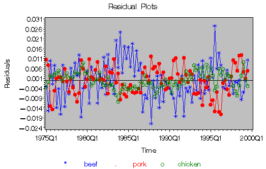Figure 7: Beef,Pork,and Chicken Residuals

The estimated parameters are stored in data sets and will be used in calculating price and income elasticities in the example "Calculating Elasticities in an Almost Ideal Demand System."

Acknowledgment

The SAS program used in this example is based on code provided by Dr. Barry Goodwin.

References

Deaton, A., and Muellbauer, J. (1980a), "An Almost Ideal Demand System," American Economic Review, 70, 312-336.

Deaton, A., and Muellbauer, J. (1980b), Economics and Consumer Behavior, Cambridge, England: Cambridge University Press.

Piggott, N. (1997), The Benefits and Costs of Generic Advertising of Agricultural Commodities, Ph.D. dissertation, University of California, Davis.

SAS Institute Inc. (1999), SAS/ETS User's Guide, Version 8, Cary, NC: SAS Institute Inc.

USDA-ERS Electronic Data Archive, Red Meats Yearbook, housed at Cornell University's Mann Library, [http://usda.mannlib.cornell.edu/], accessed 25 September 2001.

USDA-ERS Electronic Data Archive, Poultry Yearbook, housed at Cornell University's Mann Library, [http://usda.mannlib.cornell.edu/], accessed 25 September 2001.

These sample files and code examples are provided by SAS Institute Inc. "as is" without warranty of any kind, either express or implied, including but not limited to the implied warranties of merchantability and fitness for a particular purpose. Recipients acknowledge and agree that SAS Institute shall not be liable for any damages whatsoever arising out of their use of this material. In addition, SAS Institute will provide no support for the materials contained herein.

   /*-----------------------------------------------------------------
     Example: Estimating an Almost Ideal Demand System Model
     Requires: SAS/ETS
     Version: 9.0
     ------------------------------------------------------------------*/

data aids_;
   input year qtr pop beef_q pork_q chick_q turkey_q beef_p pork_p chick_p
         turkey_p cpi pc_exp;
   date = yyq(year,qtr);
   format date yyq6.;
   datalines;

1975 1 215.132 22.0991 11.8074 9.2631  1.0724 134.8333 120.8 58.9   72.13  52.43  1143.95149
1975 2 215.646 21.0304 11.0085 10.1645 1.3916 152.6333 129.8 58.97  70.83  53.23  1175.192619
1975 3 216.294 22.2717 9.6583  10.2047 1.8937 163.2    157.4 68.93  73.87  54.37  1210.389562
1975 4 216.851 22.7502 10.4302 9.7381  3.9068 158.1667 161.8 66.3   78.27  55.23  1240.483097
1976 1 217.315 23.8753 10.939  10.3294 1.145  148.7    149.4 61.93  78.1   55.77  1278.213653
1976 2 217.773 22.8964 10.3597 10.9598 1.5151 148.2    146.3 60.7   77     56.47  1298.48512
1976 3 218.337 24.4652 11.0404 11.031  2.0091 142.8    145.1 60.9   76.87  57.37  1329.141028
1976 4 218.92  23.1085 13.1403 10.1654 4.2247 142.9333 126.6 55.13  78.23  58.03  1365.909921
1977 1 219.424 22.9976 11.9593 10.3395 1.2198 142.1667 127.2 58.27  76.07  59.03  1403.219338
1977 2 219.953 22.6131 11.4488 11.2841 1.3872 143.9333 128.8 60.8   74.1   60.33  1432.468374
1977 3 220.573 23.4054 11.2324 11.1785 2.109  146.5    138.6 61.9   76.83  61.2   1464.254465
1977 4 221.206 22.7401 12.3959 10.4996 4.0197 150.8    135.7 59.3   80.42  61.87  1503.010768
1978 1 221.711 22.0441 11.6947 10.8966 1.2211 160      144.9 61.4   74.53  62.93  1533.30582
1978 2 222.278 21.7602 11.4791 11.8033 1.589  182.5333 150.7 66.93  79.6   64.53  1595.978
1978 3 222.929 21.6064 11.4611 11.6097 2.0336 186.2    153.1 70.5   84.37  66.07  1628.433268
1978 4 223.574 21.8814 12.3615 11.1396 3.88   186.4333 158.8 67.07  87.73  67.4   1666.789669
1979 1 224.144 20.5086 12.1608 11.4686 1.3533 211.7    165.1 69.6   90.33  69.07  1708.165287
1979 2 224.738 19.0408 13.1374 12.6605 1.7558 231.5    156.8 70.33  91.03  71.47  1743.033539
1979 3 225.421 19.1457 13.5239 12.582  2.1241 222.7    146   65.93  89.83  73.83  1796.749194
1979 4 226.135 19.3989 14.8575 11.6184 4.0155 223.8333 142.1 64.87  88.17  75.93  1842.372919
1980 1 226.753 18.947  14.5643 12.1178 1.7761 231.1667 141.7 67.57  92.77  78.93  1891.930629
1980 2 227.387 18.898  14.8637 12.6824 1.9508 227.5    132.5 63.53  90.2   81.83  1890.283724
1980 3 228.07  19.2127 13.5274 11.7869 2.5774 237.5333 152.6 75.07  93.63  83.33  1947.980769
1980 4 228.696 19.4988 14.3512 11.4689 3.9459 238.1667 163.2 77.27  98.17  85.53  2010.533657
1981 1 229.148 19.3429 14.0974 12.0277 1.6042 233.5    157.3 75.43  98.13  87.8   2065.37274
1981 2 229.668 18.9816 13.4164 12.6866 1.9006 230.7    153.1 71.9   98.47  89.83  2097.266489
1981 3 230.3   19.6459 13.0621 12.8079 2.4992 239.0333 166.6 74.9   101.83 92.37  2139.062395
1981 4 230.906 19.2868 14.0918 11.9454 4.5618 235.4333 167.9 70.47  92.97  93.7   2150.663367
1982 1 231.392 18.8193 12.7405 11.9425 1.7318 233.3    169.4 71.77  92.47  94.47  2185.689621
1982 2 231.901 18.7968 12.2607 12.834  2.0328 242.9667 179.2 72.13  91.3   95.9   2208.705889
1982 3 232.496 19.9882 11.5797 12.9951 2.5874 244.0333 195.7 72.33  95.47  97.7   2251.333897
1982 4 233.077 19.4242 12.5368 11.8858 4.2141 233.1333 198   69.2   92.9   97.93  2307.933232
1983 1 233.543 19.2252 12.114  12.4026 2.0296 233.8667 193.6 69.53  92.07  97.87  2342.609284
1983 2 234.02  19.3361 12.7472 13.129  2.1634 240.9333 181   68.73  92.57  99.1   2414.323562
1983 3 234.601 20.4952 12.8496 12.5883 2.4668 234.3667 175   74.43  92.7   100.27 2471.643343
1983 4 235.157 19.5995 14.0587 11.6903 4.3635 227.1667 169.1 77.17  91.33  101.17 2527.997312
1984 1 235.601 19.3191 12.8106 12.3375 1.9057 238.4667 170.9 85.13  94.33  102.3  2575.434739
1984 2 236.077 19.3744 12.6312 13.3105 2.155  238      168.7 82.4   97.2   103.4  2627.749903
1984 3 236.655 19.9738 12.3802 13.1955 2.5966 232.2    173.5 80.23  101.77 104.53 2659.045148
1984 4 237.238 19.7597 13.6804 12.6693 4.3788 233.2333 172.7 76.27  102.37 105.3  2706.148901
1985 1 237.667 19.0586 12.7537 12.7081 1.9896 234.9    175   77.13  107.23 105.97 2769.52627
1985 2 238.172 20.0757 12.855  13.7851 2.1634 230.4333 167.8 75.67  103.43 107.27 2815.297348
1985 3 238.789 20.8175 12.8035 13.5748 2.7299 222.7333 170.4 75.73  105.23 108.03 2878.907485
1985 4 239.392 19.2488 13.4707 13.0119 4.7012 226.4333 172.4 76.77  104.93 109    2909.036225
1986 1 239.858 19.0212 12.4462 13.0699 2.3152 229.2667 177.4 76.8   106.3  109.23 2944.554695
1986 2 240.365 20.1607 12.3281 14.1113 2.3758 222.9    173.2 77.2   103.3  109    2971.522476
1986 3 240.961 20.7108 11.5663 13.813  3.0149 225.6333 200.3 91.9   109    109.8  3038.458506
1986 4 241.544 18.9416 12.6462 13.2814 5.1658 229.3    204.1 88.1   107.7  110.4  3073.980463
1987 1 242.005 18.2746 12.2342 14.0183 2.5318 230.6    195.7 81.9   103.27 111.63 3110.892566
1987 2 242.516 18.5266 11.7023 14.5088 2.8807 239.1    194   78.17  102.77 113.1  3176.601083
1987 3 243.118 19.175  11.7285 14.5456 3.4995 242.1667 206.9 77.77  104.73 114.4  3234.547081
1987 4 243.724 17.8807 13.513  14.2982 5.8184 241.6667 200.7 76.1   93.97  115.37 3264.861072
1988 1 244.205 18.1678 12.8332 14.3959 3.035  241.7333 194.6 74.6   92.33  116.07 3337.155259
1988 2 244.708 18.4639 12.5507 14.7447 3.4076 250.1    195.5 80.8   91.73  117.53 3391.286758
1988 3 245.352 18.7622 12.9249 14.2711 3.7854 254.5333 196.7 95.77  98.7   119.1  3451.164042
1988 4 245.97  17.2552 14.1567 14.0575 5.4503 255      189.4 90.3   100.1  120.33 3516.790666
1989 1 246.454 16.9765 12.8213 14.3563 3.1189 260.7    190.5 90.57  97.27  121.67 3562.328061
1989 2 247.01  17.5192 13.0187 15.0116 3.2763 266.9667 188.9 95.83  99.9   123.67 3616.149144
1989 3 247.695 17.5975 12.6332 15.0852 4.1933 268.0333 194.6 95.33  103.57 124.67 3660.658594
1989 4 248.38  17.2416 13.5038 14.8018 6.0078 266.9333 199.8 89.07  96.8   125.87 3699.069973
1990 1 248.92  16.5516 12.5572 14.9451 3.5354 272.6333 207.6 90.2   98.87  128.03 3771.098689
1990 2 249.562 17.3763 11.8816 15.4012 3.6762 281.2    220.5 90.9   98.9   129.33 3812.887805
1990 3 250.301 17.4207 12.1079 15.5829 4.2115 280.3667 235.5 91.2   101.83 131.57 3866.944199
1990 4 251.04  16.4315 13.216  15.5973 6.1275 289.8667 236   87.37  97.57  133.7  3877.278277
1991 1 251.649 15.9842 12.2575 15.1466 3.6626 294.2667 227.6 89.6   99.47  134.8  3879.014024
1991 2 252.299 17.0449 12.0445 16.4942 3.9074 295.2    225.6 88.2   101.03 135.6  3922.536202
1991 3 253.041 17.5591 12.2515 16.5271 4.0353 284.6333 227   87.7   103.1  136.67 3950.158176
1991 4 253.756 16.2093 13.8041 15.8341 6.2823 279.2    216.4 86.63  95.67  137.7  3964.0442
1992 1 254.337 16.3952 13.1929 16.8084 3.4475 282.2667 210.4 86.2   95.37  138.67 4052.800129
1992 2 255.04  16.9538 12.697  17.1634 3.7342 286.8333 207.3 85.87  98.47  139.8  4089.06446
1992 3 255.832 17.227  13.2128 17.3147 4.2    282.6667 211.8 88.03  100.1  140.9  4129.378126
1992 4 256.561 15.9093 13.9768 16.4821 6.4864 286.6667 208.5 87.63  93.97  141.9  4207.876895
1993 1 257.157 15.8915 13.018  17.3378 3.5527 292.1333 205.9 87.5   99.07  143.1  4229.517377
1993 2 257.785 16.2058 12.6251 17.9871 3.7316 300.4    205.5 88.43  101.37 144.2  4287.786892
1993 3 258.511 17.043  12.8477 17.9543 3.9801 292      211.8 89.43  102.43 144.77 4340.434256
1993 4 259.177 15.9513 13.8657 16.9636 6.4533 289.2333 213.2 90.7   97.5   145.77 4397.292964
1994 1 259.65  16.2494 12.5018 17.516  3.5479 286.6667 212.5 89.27  98.5   146.7  4442.326208
1994 2 260.261 16.8868 12.9018 18.0614 3.7688 286.1667 210.4 90.63  98.83  147.63 4493.085787
1994 3 260.948 17.3775 13.1741 18.6015 4.414  279.5    210.5 90.87  102.73 148.93 4553.589221
1994 4 261.59  16.4723 14.4918 17.3363 6.1044 279.1667 204.8 89.6   100.07 149.63 4607.69641
1995 1 262.123 16.3097 13.1044 17.9111 3.5628 283.8667 202.7 90.23  99.77  150.87 4643.430756
1995 2 262.707 17.0895 12.9167 18.5493 3.9053 283.1    201.2 90.33  102.9  152.2  4704.584774
1995 3 263.396 17.647  12.6978 17.343  4.1648 285.1    206.9 92.2   106.53 152.87 4750.641619
1995 4 264.055 16.3476 13.7183 17.0398 6.173  285.2667 213.5 93.9   100.27 153.6  4789.162843
1996 1 264.535 17.0783 12.6109 18.2436 3.7235 278.7    218.3 93.8   105.03 155    4848.611429
1996 2 265.13  17.6763 11.5758 18.6502 3.9    277.4    227.4 95.47  103.27 156.53 4920.237092
1996 3 265.836 17.1606 12.0383 18.5709 4.6382 279.8    243.8 98.93  106.5  157.37 4950.138431
1996 4 266.515 16.2764 12.8608 17.486  6.206  285.0333 245.4 100.87 102.5  158.5  5007.138448
1997 1 267.032 16.2921 11.7752 17.559  3.4603 278.8    244.4 101.1  105.9  159.57 5084.418879
1997 2 267.668 17.2994 11.5617 18.7398 3.9826 278.9667 243.1 100.07 105.17 160.2  5105.49469
1997 3 268.402 17.0513 12.0187 18.4364 4.1989 281.0667 248.1 99.5   108.5  160.83 5187.275058
1997 4 269.085 16.2354 13.3464 17.635  5.9572 279.3    244.4 100.1  100.67 161.47 5231.896984
1998 1 269.583 16.6884 12.7173 17.464  3.9209 273.4667 245.6 102.03 101.03 161.9  5299.583615
1998 2 270.216 17.1985 12.3142 18.1367 3.9191 278.1    239.8 102.57 97.33  162.77 5381.075475
1998 3 270.949 17.5085 13.0799 18.5167 4.1742 277.3667 244.9 105.53 102.8  163.4  5434.243039
1998 4 271.633 16.6475 14.384  18.7589 6.0081 279.5333 240.4 107.33 97.1   163.97 5497.95128
1999 1 272.136 16.6785 13.5476 19.5127 3.84   278      235.8 106.43 98.47  164.6  5595.374363
1999 2 272.774 17.7635 13.055  19.9553 3.831  284.7667 238.4 104.13 97.2   166.2  5683.103381
1999 3 273.52  17.6689 13.218  19.2361 4.3288 289.2333 246.4 105.6  102.77 167.23 5761.655019
;
run;

   proc means data=aids_;
   run;

   data aids;
      set aids_;
      if year < 1975 then delete;
      t = _n_ ;
      co1 = cos(1/2*3.14159*t);
      co2 = cos(2/2*3.14159*t);

      si1 = sin(1/2*3.14159*t);
      si2 = sin(2/2*3.14159*t);

      x = beef_p*beef_q + pork_p*pork_q + chick_p*chick_q
          + turkey_p*turkey_q;

      w_beef = beef_p*beef_q/x;
      w_pork = pork_p*pork_q/x;
      w_chick = chick_p*chick_q/x;
      w_turkey = turkey_p*turkey_q/x;
   run;

   data aids ;
      set aids;
      obs = _n_ ;
   run;

   proc gplot data=aids;
      plot w_beef*date w_pork*date w_chick*date w_turkey*date/
           overlay cframe=ligr haxis=axis1 vaxis=axis2;
      title 'Budget Shares Plots';
      footnote1 c=blue '  *     beef   '
                c=red  '  .     pork  '
                c=green '  o    chicken  '
                c=black '  +    turkey   ';
      symbol1 c=blue i=join v=star;
      symbol2 c=red  i=join v=dot;
      symbol3 c=green i = join v = circle ;
      symbol4 c=black i = join v = plus ;
      axis1  label=('Time') ;
      axis2  label=(angle=90 'Budget Share');
   run;
   quit;
   footnote;

   proc means data=aids noprint;
      var beef_p pork_p chick_p turkey_p;
      output out=pm mean=b_m p_m c_m t_m;
   run;

   data aids ;
      if _n_ = 1 then set pm ;
      set aids ;

      pb_ = (beef_p/b_m);
      pp_ = (pork_p/p_m);
      pc_ = (chick_p/c_m);
      pt_ = (turkey_p/t_m);

      lpb = log(pb_);
      lpp = log(pp_);
      lpc = log(pc_);
      lpt = log(pt_);

      lx = log(x);

   /* Specify the linear price index for the LA-AIDS model */
      lp0 = sum(w_beef*lpb + w_pork*lpp + w_chick*lpc + w_turkey*lpt);
      lxp = lx-lp0;
   run;

   proc means noprint;
      var w_beef w_pork w_chick w_turkey pb_ pp_ pc_ pt_ x lp0;
      output out=meanw mean= w_beef w_pork w_chick w_turkey bm pm cm tm x lp0;
   run;

   /* Linear Approximate AIDS (LA-AIDS) Model*/
   proc model data=aids ;
   /*imposing homogeneity and symmetry restrictions on the parameters*/
      gbt = 0-gbb-gbp-gbc;
      gpt = 0-gbp-gpp-gpc;
      gct = 0-gbc-gpc-gcc;
   /* delete last equation(turkey) for adding up*/
      w_beef = ab + gbb*lpb + gbp*lpp + gbc*lpc + gbt*lpt + bb*lxp;
      w_pork = ap + gbp*lpb + gpp*lpp + gpc*lpc + gpt*lpt + bp*lxp;
      w_chick = ac + gbc*lpb + gpc*lpp + gcc*lpc + gct*lpt + bc*lxp;
      fit w_beef w_pork w_chick / itsur nestit outest=fin0;
      parms ab bb gbb gbp gbc
            ap bp     gpp gpc
            ac bc         gcc ;
   run;
   quit ;

   proc syslin itsur data = aids outest = fin1;
      b: model w_beef = lpb lpp lpc lpt lxp co1 si1 t ;
      p: model w_pork = lpb lpp lpc lpt lxp co1 si1 t ;
      c: model w_chick = lpb lpp lpc lpt lxp co1 si1 t ;

      srestrict
      /*symmetry restrictions */
      b.lpp = p.lpb ,
      b.lpc = c.lpb ,
      p.lpc = c.lpp ,
      /* homogeneity restrictions*/
      b.lpb + b.lpp + b.lpc + b.lpt = 0 ,
      p.lpb + p.lpp + p.lpc + p.lpt = 0 ,
      c.lpb + c.lpp + c.lpc + c.lpt = 0;
   run;

  /* Full Nonlinear AIDS Model */
   proc model data=aids;

   /* imposing homogeneity and symmetry and adding-up restrictions */
      restrict gbb + gbp + gbc + gbt = 0 ,
               gbp + gpp + gpc + gpt = 0 ,
               gbc + gpc + gcc + gct = 0 ,
               gbt + gpt + gct + gtt = 0 ,
               ab + ap + ac + at = 1 ;


   /*non-linear price index*/
      a0 = 0; /* restrict the constant term in the nonlinear price index to be zero */
      p = a0 + ab*lpb + ap*lpp + ac*lpc + at*lpt +
      .5*(gbb*lpb*lpb + gbp*lpb*lpp + gbc*lpb*lpc + gbt*lpb*lpt +
          gbp*lpp*lpb + gpp*lpp*lpp + gpc*lpp*lpc + gpt*lpp*lpt +
          gbc*lpc*lpb + gpc*lpc*lpp + gcc*lpc*lpc + gct*lpc*lpt +
          gbt*lpt*lpb + gpt*lpt*lpp + gct*lpt*lpc + gtt*lpt*lpt );

   /*share equation*/
      w_beef = ab + gbb*lpb + gbp*lpp + gbc*lpc + gbt*lpt + bb*(lx-p)
               + abco1*co1 + absi1*si1 + ab_t*t ;
      w_pork = ap + gbp*lpb + gpp*lpp + gpc*lpc + gpt*lpt + bp*(lx-p)
               + apco1*co1 + apsi1*si1 + ap_t*t ;
      w_chick = ac + gbc*lpb + gpc*lpp + gcc*lpc + gct*lpt + bc*(lx-p)
                + acco1*co1 + acsi1*si1 + ac_t*t ;

      fit w_beef w_pork w_chick / itsur nestit outs=rest estdata=fin0 outest=fin2
          out = resid2 converge = .00001  maxit = 1000 ;
      parms ab bb gbb gbp gbc gbt abco1 absi1 ab_t
            ap bp     gpp gpc gpt apco1 apsi1 ap_t
            ac bc         gcc gct acco1 acsi1 ac_t
         at                gtt ;

   run;
   quit;

   data resid2;
      merge resid2 aids_;
   run;

   proc gplot data = resid2;

      plot w_beef*date w_pork*date w_chick*date / overlay cframe=ligr
                                        haxis=axis1 vaxis=axis2 vref=0;
      title 'Residual Plots';

      footnote1 c=blue '  *     beef   '
                c=red  '  .     pork  '
                c=green '  o    chicken  ';

      symbol1 c=blue i=join v=star;
      symbol2 c=red  i=join v=dot;
      symbol3 c=green i = join v = circle ;

      axis1  label=('Time') ;
      axis2  label=(angle=90 'Residuals');
   run;
   quit;