There are several response distributions available when fitting generalized linear models (GLMs) in procedures such as GENMOD, GLIMMIX, and others. The distributions include the normal, Poisson, gamma, inverse Gaussian, Tweedie, and others. One important aspect of how these distributions differ is in the relationship between the mean and the variance. For the normal distribution, the variance is not related to the mean. The mean and variance are the same in the Poisson. In the gamma distribution, the variance is the square of the mean. The variance is the mean cubed in the inverse Gaussian. The Tweedie distribution includes a power parameter which defines a family of distributions that can have any of the above mean-variance relationships, as well as relationships in between.

When it comes to selecting a distribution to use when modeling a response, choosing a distribution that matches the observed mean-variance relationship is clearly important. Discussed below are some tools for finding a suitable response distribution if it is not already known. First, graphical methods using the observed data can be used to visually assess the nature of the relationship. Alternatively, assuming that the variance is proportional to a power of the mean, V(y)=φμ^p, then one can attempt to estimate p. One way to do this is using a modification of Park's test for heteroscedasticity. Manning and Mullahy (2001) discuss this modification of the test and its use. The idea is to use the predicted values and residuals from an initial log-linked GLM to model the variance as a function of the mean using another log-linked GLM of the form

ln(V(y)) = c + p*ln(μ)

(1)

If the estimate of p is near 0, then this suggests that a normal response is reasonable. For p near 1, the response distribution is similar to the Poisson, but continuous rather than discrete. Note that PROC GENMOD does not require that the response be discrete in order to use the Poisson response distribution. The gamma distribution is suggested for p near 2, and the inverse Gaussian for p near 3. The method assumes independent observations, that the mean model is a log-linked model, that the response is positive with no censoring or truncation, and that exposures do not vary (as when using an offset). The variance is assumed to be a function of the covariates through the mean, not directly of the covariates.

An alternative to the modified Park method is to fit the desired model using a distribution which encompasses a range of powers. The Tweedie distribution assumes that the variance is proportional to a power, p, of the mean. For p=0, 1, 2, or 3, the Tweedie is equivalent to the above distributions. But it also accommodates noninteger powers so you do not have to choose between, say, the gamma and inverse Gaussian if p=2.5. Using the Tweedie distribution, PROC GENMOD can estimate the power for p>1.1. For more information on the Tweedie distribution, see "Tweedie Distribution For Generalized Linear Models" in the Details section of the GENMOD documentation.

Examples

In the following examples, the methods discussed above are illustrated using simulated data from known distributions and mean models and also using observed data.

Gamma: p=2

The statements below produce a data set of values y_ij ~ gamma(a,λ_i), where a=e², λ_i=e^0.1x_i, i=1, 2, ..., 10, j=1, 2, ..., 1000. The ten gamma-distributed populations correspond to the levels of predictor, x_i=i. As shown in this note, the means of the populations are μ_i = aλ_i. The true log-linked model for the mean is then

log(μi) = 2 + 0.1xi

(2)

The population variances are aλ_i². Notice that the variances are proportional to the square of the means since V(y)= 1 a μ². As a result, we expect to obtain an estimate of the power, p, near 2. In the following code, the use of the STREAMINIT function allows the random stream of gamma variates and subsequent analyses to be reproduced.

      data P2; 
         call streaminit(48945);
         keep id x y; 
         a=exp(2);
         do i=1 to 10; 
            do j=1 to 1000;
               x=i;
               lambda=exp(0.1*x);
               y=lambda*rand("gamma",a); 
               id+1;
               output; 
            end;
         end;
         run;

Graphical assessment

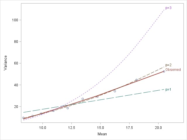
The mean-variance relationship can be assessed graphically using the following statements. For each of the Poisson, gamma, and inverse Gaussian distributions, the variance is proportional to a power of the mean with the square or reciprocal of the distribution's scale parameter as the proportionality constant. See "Generalized Linear Models Theory" in the Details section of the GENMOD documentation. To plot the mean-variance relationships under these distributions for comparison to the observed data, a model using each of the distributions is fit and the estimated scale parameter is obtained. Since the Poisson distribution does not include a scale parameter, one is added and estimated from the deviance using the SCALE=D option.

      proc genmod data=P2;
         model y=x / dist=igaussian link=log;
         run;
      proc genmod data=P2;
         model y=x / dist=gamma link=log;
         run;
      proc genmod data=P2;
         model y=x / dist=poisson link=log scale=d;
         run;

The estimated variance for each distribution is then computed for each population using the observed mean and the estimated scale.

      proc means data=P2 nway mean var min max; 
         class x; var y; 
         output out=MV2 mean=Mean var=Variance; 
         run;
      data MV2; set MV2; 
         v3=Mean**3 * 0.1128**2;   * estimate inverse Gaussian variance;
         v2=Mean**2 * (1/7.4134);  * estimate gamma variance;
         v1=Mean    * 1.3226**2;   * estimate Poisson-like variance;
         run;

Finally, these statements plot the observed means and variances and the relationships under the various distributions representing powers of the mean.

      proc sort data=MV2;
         by Mean;
         run;
      proc sgplot data=MV2 cycleattrs noautolegend; 
         loess y=Variance x=Mean / lineattrs=(thickness=2 pattern=solid) curvelabel="Observed"; 
         spline y=v1 x=Mean / lineattrs=(pattern=5) curvelabel="p=1"; 
         spline y=v2 x=Mean / lineattrs=(pattern=4) curvelabel="p=2"; 
         spline y=v3 x=Mean / lineattrs=(pattern=2) curvelabel="p=3"; 
         yaxis label="Variance";
         run;

The observed mean-variance relationship, approximated with a smoothed, loess curve through the observed values, seems closest to the p=2 curve, suggesting the gamma distribution.

Modified Park method

The method begins by estimating an initial log-linked GLM^Note1 to the data and saving the predicted values and raw residuals in a data set. The gamma distribution is used below for the initial model. To model the variance, the natural log of the predicted values and of the raw residuals are computed. PROC REG is then used to fit the variance model (1) above^Note2. The power of the mean, p, is the estimated parameter for Lnp. The CLB option provides a confidence interval for p.

      proc genmod data=P2;
         model y=x / dist=gamma link=log;
         output out=P2predres p=p resraw=rr;
         run;
      data P2predres;
         set P2predres;
         Lnp=log(p);
         Lnrr2=log(rr**2);
         run;
      proc reg data=P2predres plots=none;
         model Lnrr2 = Lnp / clb;
         run; quit;

The estimated power is 1.97 with a 95% confidence interval of (1.82, 2.12). This estimate is very near 2 as expected for gamma distributed data and is in agreement with the visual assessment above.

Parameter Estimates Variable DF Parameter Estimate Standard Error t Value Pr > |t| 95% Confidence Limits Intercept 1 -3.22424 0.19647 -16.41 <.0001 -3.60936 -2.83912 Lnp 1 1.96943 0.07656 25.72 <.0001 1.81936 2.11951

The final model then is the same as the initial gamma model above. Notice that the estimated parameters closely match the true log-linked mean model (2). The scale parameter, 7.41 = a = e² as shown in this note.

Analysis Of Maximum Likelihood Parameter Estimates Parameter DF Estimate Standard Error Wald 95% Confidence Limits Wald Chi-Square Pr > ChiSq Intercept 1 2.0041 0.0079 1.9886 2.0196 64219.5 <.0001 x 1 0.0993 0.0013 0.0968 0.1018 6082.51 <.0001 Scale 1 7.4134 0.1026 7.2151 7.6172

Tweedie model

Since the graphical assessment above suggests that the power of the mean is at least 1.1, a GLM using the Tweedie distribution can be used to simultaneously estimate the power and fit the model.

      proc genmod data=P2;
         model y=x / dist=tweedie link=log;
         run; 

The estimated power is again very close to 2 – 1.96 with 95% confidence interval (1.89, 2.03) – and the estimated parameters are essentially identical to those from the gamma model above.

Analysis Of Maximum Likelihood Parameter Estimates Parameter DF Estimate Standard Error Wald 95% Confidence Limits Wald Chi-Square Pr > ChiSq Intercept 1 2.0040 0.0079 1.9885 2.0196 63798.5 <.0001 x 1 0.0993 0.0013 0.0968 0.1018 6099.89 <.0001 Dispersion 1 0.1487 0.0140 0.1213 0.1760     Power 1 1.9605 0.0378 1.8865 2.0345

Inverse Gaussian: p=3

A data set is generated containing inverse Gaussian random values y_ij ~ IG(μ_i,σ), where μ_i=e^1+x, x=0.2, 0.4, ..., 2, and σ=1. The true log-linked model for the mean is then log(μ_i)=1+x_i. The population variances are σμ_i³, which is proportional to μ³ so the estimated power is expected to near 3.

Graphical assessment

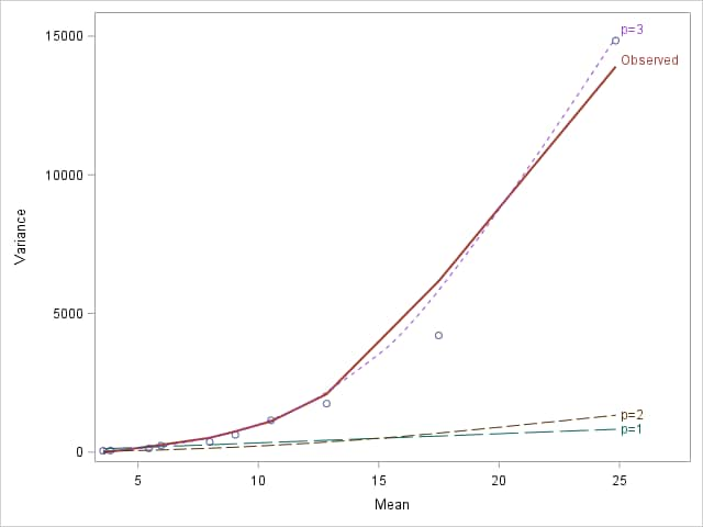
As in the previous example, models are fit to estimate the Poisson, gamma, and inverse Gaussian scale parameters and a plot is produced of the observed population means and variances along with curves showing the expected mean-variance relationships under each of those distributions. The resulting plot correctly suggests that the inverse Gaussian distribution closely approximates the observed mean-variance relationship.

Modified Park method

Applying the modified Park method as shown in the previous example, the estimated power is 2.39 with 95% confidence interval (2.33, 2.45). This suggests that the distribution is somewhere between gamma and inverse Gaussian.

Parameter Estimates Variable DF Parameter Estimate Standard Error t Value Pr > |t| 95% Confidence Limits Intercept 1 -1.41774 0.06806 -20.83 <.0001 -1.55116 -1.28433 Lnp 1 2.39376 0.03065 78.10 <.0001 2.33368 2.45384

Given that the mean-variance plot points more strongly to the inverse Gaussian, that distribution is selected for the final model. The estimated model parameters closely match the true values.

Analysis Of Maximum Likelihood Parameter Estimates Parameter DF Estimate Standard Error Wald 95% Confidence Limits Wald Chi-Square Pr > ChiSq Intercept 1 1.0262 0.0472 0.9337 1.1187 472.62 <.0001 x 1 1.0076 0.0496 0.9104 1.1047 413.24 <.0001 Scale 1 0.9880 0.0070 0.9744 1.0018

Tweedie model

Since the power of the mean-variance relationship is clearly shown by the above plot and modified Park method to be greater than 1.1, it can be estimated and the data modeled by fitting a log-linked Tweedie model in PROC GENMOD. The power estimate, 2.98 with 95% confidence interval (2.95, 3.01), is very close to its true value. The estimated parameters of the model are also very close to their true values.

Analysis Of Maximum Likelihood Parameter Estimates Parameter DF Estimate Standard Error Wald 95% Confidence Limits Wald Chi-Square Pr > ChiSq Intercept 1 1.0258 0.0465 0.9346 1.1170 485.79 <.0001 x 1 1.0081 0.0486 0.9129 1.1033 430.69 <.0001 Dispersion 1 0.9813 0.0143 0.9533 1.0094     Power 1 2.9790 0.0144 2.9509 3.0071

Baseball salary data

The sashelp.baseball data set contains salary and performance information for Major League Baseball players (excluding pitchers) who played at least one game in both the 1986 and 1987 seasons. The salaries are for the 1987 season (Sports Illustrated, April 20, 1987), and the performance measures are from the 1986 season (Collier Books, The 1987 Baseball Encyclopedia Update). Salaries will be modeled as a function of several predictors – League, Division, career runs (CrRuns), number of times at bat (nAtBat), number of hits (nHits), and number of outs (nOuts). An appropriate response distribution must be chosen for the log-linked model that will be fit.

Graphical assessment

Graphical assessment proceeds similarly to the first example above. First, the p=1, 2, and 3 models are fit to obtain their scale parameters for use in computing the variances under the three distributions.

      proc genmod data=sashelp.baseball;
         class League Division;
         model Salary=League Division CrRuns nAtBat nHits nOuts / dist=igaussian link=log;
         run;
      proc genmod data=sashelp.baseball;
         class League Division;
         model Salary=League Division CrRuns nAtBat nHits nOuts / dist=gamma link=log;
         run;
      proc genmod data=sashelp.baseball;
         class League Division;
         model Salary=League Division CrRuns nAtBat nHits nOuts / dist=poisson link=log scale=d;
         run;

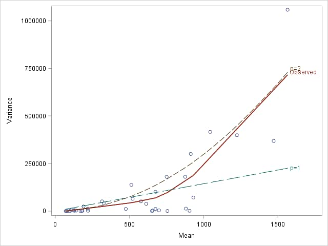
Since the continuous predictors have a large number of distinct values, they are each categorized into quintiles using PROC RANK before the means and variances of the resulting populations are computed and plotted. The observed mean-variance relationship was found not to be close to cubic, so only curves for p=1 and 2 are shown in the plot.

      proc rank data=sashelp.baseball out=rankbb groups=5; 
         var CrRuns nAtBat nHits nOuts; 
         run;
      proc means data=rankbb nway mean var min max; 
         class League Division CrRuns nAtBat nHits nOuts; 
         var salary; 
         output out=obsmv mean=Mean var=Variance; 
         run;
      data obsmv; set obsmv;
         where Variance ne .;
         v3=Mean**3 * 0.0285**2;   * estimate inverse Gaussian variance;
         v2=Mean**2 * (1/3.3558);  * estimate gamma variance;
         v1=Mean    * 12.0001**2;  * estimate Poisson-like variance;
         run;
      proc sort data=obsmv;
         by Mean;
         run;
      proc sgplot data=obsmv cycleattrs noautolegend;  
         loess y=Variance x=Mean / lineattrs=(thickness=2 pattern=solid) curvelabel="Observed";
         spline y=v1 x=Mean / lineattrs=(pattern=5) curvelabel="p=1"; 
         spline y=v2 x=Mean / lineattrs=(pattern=4) curvelabel="p=2"; 
         yaxis label="Variance";
         xaxis label="Mean";
         run;

The plot suggests the mean-variance relationship is close to quadratic, so the gamma distribution seems reasonable.

Modified Park method

As before, an initial log-linked gamma model is used to obtain predicted and residual values which are then transformed and modeled to estimate the power of the mean-variance relationship.

      proc genmod data=sashelp.baseball;
         class League Division;
         model Salary=League Division CrRuns nAtBat nHits nOuts / dist=g link=log;
         output out=bb p=p resraw=rr;
         run;
      data bb;
         set bb;
         Lnp=log(p);
         Lnrr2=log(rr**2);
         run;
      proc reg data=bb plots=none;
         model Lnrr2 = Lnp / clb;
         run; quit;

The estimated power, p=1.80 (1.45, 2.14), agrees that the relationship is approximately quadratic.

Parameter Estimates Variable DF Parameter Estimate Standard Error t Value Pr > |t| 95% Confidence Limits Intercept 1 -1.03688 1.07759 -0.96 0.3368 -3.15876 1.08500 Lnp 1 1.79623 0.17605 10.20 <.0001 1.44957 2.14290

These statements fit the suggested gamma model and produce the following results.

      proc genmod data=sashelp.baseball;
         class League Division;
         model Salary=League Division CrRuns nAtBat nHits nOuts / dist=g link=log;
         run;

Analysis Of Maximum Likelihood Parameter Estimates Parameter   DF Estimate Standard Error Wald 95% Confidence Limits Wald Chi-Square Pr > ChiSq Intercept   1 4.7802 0.1202 4.5447 5.0157 1582.77 <.0001 League American 1 -0.1419 0.0687 -0.2764 -0.0073 4.27 0.0388 League National 0 0.0000 0.0000 0.0000 0.0000 . . Division East 1 0.1152 0.0685 -0.0191 0.2495 2.83 0.0926 Division West 0 0.0000 0.0000 0.0000 0.0000 . . CrRuns   1 0.0015 0.0001 0.0013 0.0018 141.47 <.0001 nAtBat   1 -0.0009 0.0009 -0.0027 0.0009 1.00 0.3171 nHits   1 0.0093 0.0029 0.0036 0.0150 10.13 0.0015 nOuts   1 0.0004 0.0001 0.0001 0.0006 8.71 0.0032 Scale   1 3.3558 0.2793 2.8507 3.9504

Tweedie model

Since the power is clearly larger than 1.1, the Tweedie model can be used. The Tweedie model estimates the power to be p=2.17 (1.82, 2.5) also suggesting a gamma model.

      proc genmod data=sashelp.baseball;
         class League Division;
         model Salary=League Division CrRuns nAtBat nHits nOuts / dist=tweedie link=log;
         run;

The Tweedie model with its estimated power is similar to the above gamma model.

Analysis Of Maximum Likelihood Parameter Estimates Parameter   DF Estimate Standard Error Wald 95% Confidence Limits Wald Chi-Square Pr > ChiSq Intercept   1 4.7552 0.1242 4.5117 4.9986 1465.34 <.0001 League American 1 -0.1507 0.0701 -0.2881 -0.0134 4.63 0.0315 League National 0 0.0000 0.0000 0.0000 0.0000 . . Division East 1 0.1016 0.0710 -0.0376 0.2408 2.05 0.1527 Division West 0 0.0000 0.0000 0.0000 0.0000 . . CrRuns   1 0.0017 0.0002 0.0012 0.0022 50.98 <.0001 nAtBat   1 -0.0009 0.0009 -0.0028 0.0009 1.01 0.3159 nHits   1 0.0092 0.0030 0.0033 0.0152 9.18 0.0024 nOuts   1 0.0004 0.0001 0.0001 0.0007 8.12 0.0044 Dispersion   1 0.1127 0.1143 -0.1113 0.3367     Power   1 2.1654 0.1726 1.8271 2.5037

__________

Note 1: Simulation results shown in Manning and Mullahy (2001) suggest that the distribution used for this tentative initial model is not critical. However, it might be advisable to try the method using other distributions in the initial model to see if the estimated power changes substantially.

Note 2: An alternative version of the modified Park method fits a log-linked model using GEE estimation (REPEATED statement in PROC GENMOD) to model the squared raw residuals from the initial model as a function of the log predicted values.

 

Reference

Manning, W.G., Mullahy, J. (2001). Estimating log models: to transform or not to transform? Journal of Health Economics. 20(4), 461-494.

Operating System and Release Information

Product Family	Product	System	SAS Release
			Reported	Fixed*
SAS System	SAS/STAT	z/OS
		z/OS 64-bit
		OpenVMS VAX
		Microsoft® Windows® for 64-Bit Itanium-based Systems
		Microsoft Windows Server 2003 Datacenter 64-bit Edition
		Microsoft Windows Server 2003 Enterprise 64-bit Edition
		Microsoft Windows XP 64-bit Edition
		Microsoft® Windows® for x64
		OS/2
		Microsoft Windows 8 Enterprise 32-bit
		Microsoft Windows 8 Enterprise x64
		Microsoft Windows 8 Pro 32-bit
		Microsoft Windows 8 Pro x64
		Microsoft Windows 8.1 Enterprise 32-bit
		Microsoft Windows 8.1 Enterprise x64
		Microsoft Windows 8.1 Pro 32-bit
		Microsoft Windows 8.1 Pro x64
		Microsoft Windows 10
		Microsoft Windows 95/98
		Microsoft Windows 2000 Advanced Server
		Microsoft Windows 2000 Datacenter Server
		Microsoft Windows 2000 Server
		Microsoft Windows 2000 Professional
		Microsoft Windows NT Workstation
		Microsoft Windows Server 2003 Datacenter Edition
		Microsoft Windows Server 2003 Enterprise Edition
		Microsoft Windows Server 2003 Standard Edition
		Microsoft Windows Server 2003 for x64
		Microsoft Windows Server 2008
		Microsoft Windows Server 2008 R2
		Microsoft Windows Server 2008 for x64
		Microsoft Windows Server 2012 Datacenter
		Microsoft Windows Server 2012 R2 Datacenter
		Microsoft Windows Server 2012 R2 Std
		Microsoft Windows Server 2012 Std
		Microsoft Windows XP Professional
		Windows 7 Enterprise 32 bit
		Windows 7 Enterprise x64
		Windows 7 Home Premium 32 bit
		Windows 7 Home Premium x64
		Windows 7 Professional 32 bit
		Windows 7 Professional x64
		Windows 7 Ultimate 32 bit
		Windows 7 Ultimate x64
		Windows Millennium Edition (Me)
		Windows Vista
		Windows Vista for x64
		64-bit Enabled AIX
		64-bit Enabled HP-UX
		64-bit Enabled Solaris
		ABI+ for Intel Architecture
		AIX
		HP-UX
		HP-UX IPF
		IRIX
		Linux
		Linux for x64
		Linux on Itanium
		OpenVMS Alpha
		OpenVMS on HP Integrity
		Solaris
		Solaris for x64
		Tru64 UNIX

* For software releases that are not yet generally available, the Fixed Release is the software release in which the problem is planned to be fixed.

---

When specifying a response distribution for a GLM, it is important to match the observed mean-variance relationship. With many distributions available, the graphical, modified Park, and Tweedie-based methods discussed can help to select one that is appropriate.

Type:	Usage Note
Priority:
Topic:	Analytics ==> Regression SAS Reference ==> Procedures ==> GENMOD SAS Reference ==> Procedures ==> GLIMMIX SAS Reference ==> Procedures ==> HPGENSELECT

Date Modified:	2017-04-21 14:19:52
Date Created:	2017-04-21 13:58:25