Sample 59779: Calculating Price Elasticity of Demand
 |  |  |  |
Overview
|
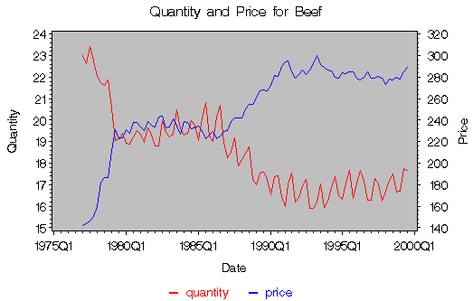
Figure 1: Quantity and Price for Beef
The price elasticity of demand is defined as the percentage change in quantity demanded for some good with respect to a one percent change in the price of the good. For example, if the price of some good goes up by 1%, and as a result sales fall by 1.5%, the price elasticity of demand for this good is -1.5%/1% = -1.5. Thus, price elasticity measures responsiveness of quantity demanded to changes in price. Price elasticity greater than one is called price elastic, and price elasticity less than one is called price inelastic. A given percentage increase in the price of an elastic good will reduce the quantity demanded for the good by a higher percentage than for an inelastic good. In general, a necessary good is less elastic than a luxury good. For an introductory text on price elasticities, see Nicholson (1992). Price elasticity can be expressed as:
where ![]() is the price elasticity,
P is the price of the good, and Q is the quantity
demanded for the good.
is the price elasticity,
P is the price of the good, and Q is the quantity
demanded for the good.
Analysis
In this example, you will calculate the price elasticity of demand for beef in a simple log-linear demand model. The data consist of quarterly retail prices and per capita consumption for beef. The data period covers the first quarter of 1977 through the third quarter of 1999. The data were obtained from the USDA Red Meats Yearbook (accessed 2001).
The log-linear demand model is of the following form:
- lnQ = a + b·lnP
where Q and P are defined as before, a and b are parameters to be estimated.
The log-linear demand model is a very simple one. In the real world, there may be many additional complexities that need to be considered in the model. For example, prices of some other closely related goods may have a significant effect on the quantity demanded for beef; hence, they may also enter the right-hand side of the demand equation. On a store level, there may also be occasions when sales remain zero regardless of how much the price is; for example, when the good is out of stock. For demonstration purposes these complexities will be ignored.
The log-linear demand function implies that the price elasticity of demand is constant:
Thus, to obtain an estimate of the price elasticity, you just need an estimate of b. You can use the AUTOREG procedure to obtain the estimates.
To use the AUTOREG procedure, you first read in the price and quantity data in the DATA step, and transform the price and quantity data into log forms:
      data a ;
         input yr qtr q p ;
         date = yyq(yr,qtr) ;
         format date yyq6. ;
         lq = log(q) ;
         lp = log(p) ;
         datalines;
      1977   1   22.9976   142.1667
      1977   2   22.6131   143.9333
      1977   3   23.4054   146.5
      1977   4   22.7401   150.8
      1978   1   22.0441   160


   ... more datalines ...

      1997   4   16.2354   279.3
      1998   1   16.6884   273.4667
      1998   2   17.1985   278.1
      1998   3   17.5085   277.3667
      1998   4   16.6475   279.5333
      1999   1   16.6785   278
      1999   2   17.7635   284.7667
      1999   3   17.6689   289.2333
      ;
      run ;
Then you specify the input data set in the PROC AUTOREG statement and specify the regression model in a MODEL statement. If you are not concerned with autocorrelated errors and just want to do an ordinary least-squares regression, you can specify the model as follows:
    proc autoreg data=a outest=estb ;
      model lq = lp ;
      output out=out1 r=resid1 ;
   title "OLS Estimates";
   run ;
This will yield ordinary least squares estimates of a and b. The output is shown in Figure 2.
Figure 2: OLS EsimatesThe parameter estimate for b is equal to -0.5314, which suggests that increasing the price for beef by 1% will reduce the demand for beef by 0.53%.
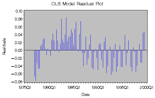
The following SAS code uses the GPLOT procedure to plot the residuals obtained from the OLS estimation, as shown in Figure 3.
    proc gplot data=plot2 ;
        title 'OLS Model Residual Plot' ;
        axis1 label=(angle=90 'Residuals') ;
        axis2 label=('Date') ;
        symbol1 c=blue i=needle v=none ;
        plot resid1*date / cframe=ligr haxis=axis2 vaxis=axis1 ;
    run ;
|
Figure 3: OLS Model Residual Plot
Note that the residual errors from the OLS regression do not appear to be random. The residual plot shows evidence of autocorrelation in the error process. This violates the independent error assumption of the classical regression model, and the OLS estimates will be inefficient. Thus, the parameter estimates are not as accurate as they could be.
To improve the efficiency of the estimated parameters, you can correct for autocorrelation using the AUTOREG procedure. Specify the order of autocorrelation using the NLAG= option. Since the data are quarterly, this example chooses order 1 as well as order 4 for seasonality considerations. You can use the METHOD= option to specify the maximum likelihood estimation.
   proc autoreg data=a outest=estb ;
      model lq = lp  / nlag=(1 4) method=ml ;
      output out=out2 r=resid2 ;
   title "OLS, Autocorrelations, & Maximum Likelihood Estimates";
   run ;
The output in Figure 4 first shows the initial OLS results. Then the estimates of autocorrelations and the maximum likelihood estimates are displayed.
The AUTOREG Procedure
The AUTOREG Procedure
|
||||||||||||||||||||||||||||||||||||||||||||||||||||||||||||||||||||||||||||||||||||||||||||||||||||||||||||||||||||||||||||||
By including an autoregressive error structure in the model, the total R2 statistic increases from 0.8521 to 0.9422 in the maximum likelihood estimation. The information criteria AIC and SBC become more negative. These imply significant improvement over the OLS estimation.
Notice also that the estimate for b changes from -0.5314 to -0.4131, which means that the estimated elasticity for beef demand is smaller in absolute value than the OLS estimate. Since the estimated elasticity is smaller than 1 in absolute value, you may conclude that demand for beef is relatively inelastic.
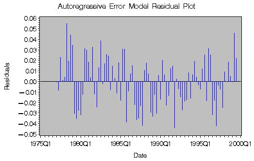
Figure 5 illustrates the residuals obtained from the autoregressive error model estimation.
    proc gplot data=plot2 ;
        title 'Autoregressive Error Model Residual Plot' ;
        axis1 label=(angle=90 'Residuals') ;
        axis2 label=('Date') ;
        symbol1 c=blue i=needle v=none ;
        plot resid2*date / cframe=ligr haxis=axis2 vaxis=axis1 ;
    run ;
|
Figure 5: Autoregressive Error Model Residual Plot
References
Nicholson, W. (1992), Microeconomic Theory: Basic Principles and Extensions, Fifth Edition, Fort Worth: Dryden Press.
SAS Institute Inc. (1999), SAS/ETS User's Guide, Version 8, Cary, NC: SAS Institute Inc.
USDA-ERS Electronic Data Archive, Red Meats Yearbook, housed at Cornell University's Mann Library, [http://usda.mannlib.cornell.edu/], accessed 25 September 2001.
These sample files and code examples are provided by SAS Institute Inc. "as is" without warranty of any kind, either express or implied, including but not limited to the implied warranties of merchantability and fitness for a particular purpose. Recipients acknowledge and agree that SAS Institute shall not be liable for any damages whatsoever arising out of their use of this material. In addition, SAS Institute will provide no support for the materials contained herein.
   /*-----------------------------------------------------------------
     Example: Calculating Price Elasticity of Demand
     Requires: SAS/ETS, SAS/IML
     Version: 9.0
     ------------------------------------------------------------------*/

   data a ;
      input yr qtr q p ;
      date = yyq(yr,qtr) ;
      format date yyq6. ;
      lq = log(q) ;
      lp = log(p) ;
      datalines;
   1977   1   22.9976   142.1667
   1977   2   22.6131   143.9333
   1977   3   23.4054   146.5
   1977   4   22.7401   150.8
   1978   1   22.0441   160
   1978   2   21.7602   182.5333
   1978   3   21.6064   186.2
   1978   4   21.8814   186.4333
   1979   1   20.5086   211.7
   1979   2   19.0408   231.5
   1979   3   19.1457   222.7
   1979   4   19.3989   223.8333
   1980   1   18.947    231.1667
   1980   2   18.898    227.5
   1980   3   19.2127   237.5333
   1980   4   19.4988   238.1667
   1981   1   19.3429   233.5
   1981   2   18.9816   230.7
   1981   3   19.6459   239.0333
   1981   4   19.2868   235.4333
   1982   1   18.8193   233.3
   1982   2   18.7968   242.9667
   1982   3   19.9882   244.0333
   1982   4   19.4242   233.1333
   1983   1   19.2252   233.8667
   1983   2   19.3361   240.9333
   1983   3   20.4952   234.3667
   1983   4   19.5995   227.1667
   1984   1   19.3191   238.4667
   1984   2   19.3744   238
   1984   3   19.9738   232.2
   1984   4   19.7597   233.2333
   1985   1   19.0586   234.9
   1985   2   20.0757   230.4333
   1985   3   20.8175   222.7333
   1985   4   19.2488   226.4333
   1986   1   19.0212   229.2667
   1986   2   20.1607   222.9
   1986   3   20.7108   225.6333
   1986   4   18.9416   229.3
   1987   1   18.2746   230.6
   1987   2   18.5266   239.1
   1987   3   19.175    242.1667
   1987   4   17.8807   241.6667
   1988   1   18.1678   241.7333
   1988   2   18.4639   250.1
   1988   3   18.7622   254.5333
   1988   4   17.2552   255
   1989   1   16.9765   260.7
   1989   2   17.5192   266.9667
   1989   3   17.5975   268.0333
   1989   4   17.2416   266.9333
   1990   1   16.5516   272.6333
   1990   2   17.3763   281.2
   1990   3   17.4207   280.3667
   1990   4   16.4315   289.8667
   1991   1   15.9842   294.2667
   1991   2   17.0449   295.2
   1991   3   17.5591   284.6333
   1991   4   16.2093   279.2
   1992   1   16.3952   282.2667
   1992   2   16.9538   286.8333
   1992   3   17.227    282.6667
   1992   4   15.9093   286.6667
   1993   1   15.8915   292.1333
   1993   2   16.2058   300.4
   1993   3   17.043    292
   1993   4   15.9513   289.2333
   1994   1   16.2494   286.6667
   1994   2   16.8868   286.1667
   1994   3   17.3775   279.5
   1994   4   16.4723   279.1667
   1995   1   16.3097   283.8667
   1995   2   17.0895   283.1
   1995   3   17.647    285.1
   1995   4   16.3476   285.2667
   1996   1   17.0783   278.7
   1996   2   17.6763   277.4
   1996   3   17.1606   279.8
   1996   4   16.2764   285.0333
   1997   1   16.2921   278.8
   1997   2   17.2994   278.9667
   1997   3   17.0513   281.0667
   1997   4   16.2354   279.3
   1998   1   16.6884   273.4667
   1998   2   17.1985   278.1
   1998   3   17.5085   277.3667
   1998   4   16.6475   279.5333
   1999   1   16.6785   278
   1999   2   17.7635   284.7667
   1999   3   17.6689   289.2333
   ;
   run ;


    proc autoreg data=a outest=estb ;
      model lq = lp ;
      output out=out1 r=resid1 ;
   title "OLS Estimates";
   run ;


   proc autoreg data=a outest=estb ;
      model lq = lp  / nlag=(1 4) method=ml ;
      output out=out2 r=resid2 ;
   title "OLS, Autocorrelations, & ML";
   run ;


    data plot2 ;
       merge out1 out2 a ;
    run ;


    proc gplot data=plot2 ;
        title 'OLS Model Residual Plot' ;
        axis1 label=(angle=90 'Residuals') ;
        axis2 label=('Date') ;
        symbol1 c=blue i=needle v=none ;
        plot resid1*date / cframe=ligr haxis=axis2 vaxis=axis1 ;
    run ;


   proc autoreg data=a outest=estb ;
      model lq = lp  / nlag=(1 4) method=ml ;
      output out=out2 r=resid2 ;
   title "OLS, Autocorrelations, & Maximum Likelihood Estimates";
   run ;


    proc gplot data=plot2 ;
        title 'Autoregressive Error Model Residual Plot' ;
        axis1 label=(angle=90 'Residuals') ;
        axis2 label=('Date') ;
        symbol1 c=blue i=needle v=none ;
        plot resid2*date / cframe=ligr haxis=axis2 vaxis=axis1 ;
    run ;


   proc iml ;
      use estb ;
      read all var {intercept lp} ;
      close estb ;
      x = (100:300)` ;
      x = log(x) ;
      y = intercept + lp*x ;
      all = y || x ;
      create outset from all ;
      append        from all ;
      quit ;
   data plot ;
       set outset(rename=(col1=y col2=x)) ;
   run ;
   proc gplot data=plot ;
      title 'Demand for Beef' ;
      axis1 label=(angle=90 'log of quantity') ;
      axis2 label=('log of price') ;
      symbol color=blue interpol=join value=none ;
      plot y*x / cframe=ligr vaxis=axis1 haxis=axis2 ;
   run ;
These sample files and code examples are provided by SAS Institute Inc. "as is" without warranty of any kind, either express or implied, including but not limited to the implied warranties of merchantability and fitness for a particular purpose. Recipients acknowledge and agree that SAS Institute shall not be liable for any damages whatsoever arising out of their use of this material. In addition, SAS Institute will provide no support for the materials contained herein.
| Type: | Sample |
| Date Modified: | 2017-01-24 12:13:50 |
| Date Created: | 2017-01-24 12:09:48 |
Operating System and Release Information
| Product Family | Product | Host | SAS Release | |
| Starting | Ending | |||
| SAS System | SAS/ETS | z/OS | ||
| z/OS 64-bit | ||||
| OpenVMS VAX | ||||
| Microsoft® Windows® for 64-Bit Itanium-based Systems | ||||
| Microsoft Windows Server 2003 Datacenter 64-bit Edition | ||||
| Microsoft Windows Server 2003 Enterprise 64-bit Edition | ||||
| Microsoft Windows XP 64-bit Edition | ||||
| Microsoft® Windows® for x64 | ||||
| OS/2 | ||||
| Microsoft Windows 8 Enterprise 32-bit | ||||
| Microsoft Windows 8 Enterprise x64 | ||||
| Microsoft Windows 8 Pro 32-bit | ||||
| Microsoft Windows 8 Pro x64 | ||||
| Microsoft Windows 8.1 Enterprise 32-bit | ||||
| Microsoft Windows 8.1 Enterprise x64 | ||||
| Microsoft Windows 8.1 Pro 32-bit | ||||
| Microsoft Windows 8.1 Pro x64 | ||||
| Microsoft Windows 10 | ||||
| Microsoft Windows 95/98 | ||||
| Microsoft Windows 2000 Advanced Server | ||||
| Microsoft Windows 2000 Datacenter Server | ||||
| Microsoft Windows 2000 Server | ||||
| Microsoft Windows 2000 Professional | ||||
| Microsoft Windows NT Workstation | ||||
| Microsoft Windows Server 2003 Datacenter Edition | ||||
| Microsoft Windows Server 2003 Enterprise Edition | ||||
| Microsoft Windows Server 2003 Standard Edition | ||||
| Microsoft Windows Server 2003 for x64 | ||||
| Microsoft Windows Server 2008 | ||||
| Microsoft Windows Server 2008 R2 | ||||
| Microsoft Windows Server 2008 for x64 | ||||
| Microsoft Windows Server 2012 Datacenter | ||||
| Microsoft Windows Server 2012 R2 Datacenter | ||||
| Microsoft Windows Server 2012 R2 Std | ||||
| Microsoft Windows Server 2012 Std | ||||
| Microsoft Windows XP Professional | ||||
| Windows 7 Enterprise 32 bit | ||||
| Windows 7 Enterprise x64 | ||||
| Windows 7 Home Premium 32 bit | ||||
| Windows 7 Home Premium x64 | ||||
| Windows 7 Professional 32 bit | ||||
| Windows 7 Professional x64 | ||||
| Windows 7 Ultimate 32 bit | ||||
| Windows 7 Ultimate x64 | ||||
| Windows Millennium Edition (Me) | ||||
| Windows Vista | ||||
| Windows Vista for x64 | ||||
| 64-bit Enabled AIX | ||||
| 64-bit Enabled HP-UX | ||||
| 64-bit Enabled Solaris | ||||
| ABI+ for Intel Architecture | ||||
| AIX | ||||
| HP-UX | ||||
| HP-UX IPF | ||||
| IRIX | ||||
| Linux | ||||
| Linux for x64 | ||||
| Linux on Itanium | ||||
| OpenVMS Alpha | ||||
| OpenVMS on HP Integrity | ||||
| Solaris | ||||
| Solaris for x64 | ||||
| Tru64 UNIX | ||||