59222 - Bayesian Quantile Regression

Sample 59222: Bayesian Quantile Regression

PDF of Example | SAS/STAT Focus Area Examples

Overview

This example demonstrates how to perform Bayesian quantile regression by using SAS/STAT software’s MCMC procedure.

Quantile regression is a technique for estimating conditional quantile functions. With quantile regression, you can model any location within a distribution, and you can estimate a set of quantiles and produce a complete picture of the covariate effect. These capabilities enable you to answer questions about how changes in the covariates affect the location, scale, and shape of a response variable’s distribution. For a Bayesian approach to quantile regression, you form the likelihood function based on the asymmetric Laplace distribution, regardless of the actual distribution of the data. In general, you can choose any prior for the quantile regression parameters, but it has been shown that the use of improper uniform priors produces a proper joint posterior distribution (Yu and Moyeed, 2001).

Analysis

The pth regression quantile $(0 < p < 1)$ is defined as any solution, $\hat{\beta }(p)$ , to the quantile regression minimization problem

$\min _{\bbeta } \sum _{t}\rho (y_{t} - \mb {x}^{\prime }_{t}{\bbeta })$

where the loss function

$\begin{align*} \rho (u) & = u(p - I(u < 0)) \\ & = u(pI(u > 0) - (1-p)I(u < 0)) \\ & = \frac{|u| + (2p - 1)u}{2} \end{align*}$

Minimization of the loss function $\rho (u)$ is equivalent to the maximization of a likelihood function formed by combining independently distributed asymmetric Laplace densities (Yu and Moyeed, 2001).

The asymmetric Laplace distribution has the following probability density function (Yu and Zhang, 2005):

$f(y; \mu , \sigma , p) = \frac{p(1-p)}{\sigma }\exp \left\{ -\rho \left(\frac{y-\mu }{\sigma }\right) \right\}$

Given the observations $\mb {y}=(y_1, \dots , y_ n)$ , the posterior distribution of $\bbeta$ , $\pi (\bbeta | \mb {y})$ is given by

$\pi (\bbeta |\mb {y}) \propto L(\mb {y}|\bbeta )g(\bbeta )$

where $g(\bbeta )$ is the prior distribution of $\bbeta$ and $L(\mb {y}|\bbeta )$ is the likelihood function, written as

$L(\mb {y}|\bbeta ) = p^ n{(1-p)}^ n \exp \left\{ -\rho (y_ i - \mb {x}_{i}^{\prime }\bbeta ) \right\}$

There is no standard conjugate prior distribution for the parameters of the pth regression quantile, but you can use Markov chain Monte Carlo (MCMC) methods to approximate the posterior distributions of the unknown parameters. Yu and Moyeed (2001) prove that if you choose the prior of $\bbeta$ to be improper uniform, then the resulting joint posterior distribution is proper.

Fitting a Single Quantile Regression Function

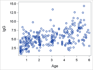
This example from Yu and Moyeed (2001) explores the distribution of the serum concentration (grams per liter) of immunoglobulin-G (IgG) conditional on age in a sample of 298 children. A detailed discussion of the data appears in Isaacs et al. (1983) and Royston and Altman (1994). The following DATA step reads the data and creates the data set Igg:


data igg;
  input IgG Age;
  Age2=age*age;
  datalines;
      1.5         .5
      2.7         .5
      1.9         .5

   ... more lines ...

      7.6   5.916667
      3.1          6
      6.8          6
;
run;

You can use the SGPLOT procedure as follows to generate a histogram of the response variable IgG for a visual inspection of its marginal distribution:


ods graphics on;
proc sgplot data=igg;
  histogram igg / nbins=50;
run;

Figure 1 shows the distribution of IgG. The distribution is asymmetric and skewed to the right.

Figure 1: Distribution of IgG

You can also use PROC SGPLOT as follows to generate a scatterplot of IgG by Age:


proc sgplot data=igg;
  scatter x=Age y=IgG;
run;

Figure 2 shows the relationship between IgG and Age. There is some evidence of an upward trend.

Figure 2: IgG by Age

Yu and Moyeed (2001) fit a quantile regression model of the form

$q_ p(IgG|Age) = \beta _0(p) + \beta _1(p)*Age + \beta _2(p)*{Age}^2$

The following SAS statements demonstrate how to use the MCMC procedure to fit this quantile regression model for a single quantile. Because PROC MCMC does not recognize the asymmetric Laplace distribution, you must write out the log-likelihood function and use the GENERAL() function.

The PROPCOV option in the PROC MCMC statement specifies that the conjugate-gradient method be used in constructing the initial covariance matrix for the Metropolis-Hastings algorithm. The NTU= option requests 1,000 tuning iterations. Experience shows that increasing the number of tuning iterations often results in improved mixing of the Markov chains. The MINTUNE= option requests a minimum of 10 proposal tuning loops. Increasing the minimum number of proposal tuning loops above the default number of 2 is sometimes needed in order to achieve convergence of the Markov chain. The NMC= option requests 30,000 MCMC iterations, excluding the burn-in iterations.

The BEGINCNST and ENDCNST statements define a statement block within which PROC MCMC processes the programming statements only during the setup stage of the simulation. You can use the BEGINCNST and ENDCNST statement block to define the constant $p$ , the quantile that is being fitted.

The PARMS statement lists the model parameters, b0, b1, and b2, and specifies that their initial values be 0.

The PRIOR statement specifies that the parameters b0, b1, and b2 have independent, improper uniform prior distributions.

The next three statements define the log-likelihood of the quantile regression model. The first and second statements are for convenience in writing the third statement. The first statement defines Mu, the location parameter of the asymmetric Laplace distribution. The second statement defines the random variable u, which is equal to the response variable IgG minus the location parameter Mu. The third statement defines the log-likelihood function in terms of the quantile $p$ and the random variable u.

The MODEL statement specifies that the response variable IgG have an asymmetric Laplace distribution, as defined by the log-likelihood function LL.


proc mcmc data=igg
          seed=5263
          propcov=congra
          ntu=1000
          mintune=10
          nmc=30000;
  begincnst;
    p=0.95;
  endcnst;
  parms (b0-b2) 0;
  prior b: ~ general(0);
  mu= b0 + b1*age + b2*age2;
  u = igg - mu;
  ll = log(p)+log(1-p) - 0.5*(abs(u)+(2*p-1)*u);
  model igg ~ general(ll);
run;

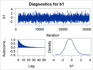
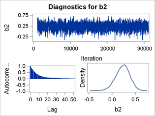
Figure 3 shows the trace plots, autocorrelation plots, and kernel density estimates of the parameters b0, b1, and b2, respectively. All three trace plots indicate convergence of the Markov chain. The autocorrelation plots show evidence of autocorrelation in the posterior samples, which often indicates slow mixing. The kernel density estimates are unimodal and relatively smooth.

Figure 3: PROC MCMC Diagnostic Plots

Output 1 shows that the Monte Carlo standard errors (MCSE) of each parameter are small relative to the posterior standard deviations (SD). A small MCSE/SD ratio indicates that the Markov chain has stabilized and the mean estimates do not vary much over time.

Output 1: Monte Carlo Standard Errors

The MCMC Procedure

Monte Carlo Standard Errors
Parameter	MCSE	Standard Deviation	MCSE/SD
b0	0.0307	1.1056	0.0277
b1	0.0245	0.9086	0.0269
b2	0.00350	0.1488	0.0235

Output 2 shows the “Effective Sample Sizes” table. The autocorrelation times for the three parameters range from 16.59 to 23.08, and the efficiency rates are low. These results account for the relatively small effective sample sizes, given a nominal sample size of 30,000.

Output 2: Effective Sample Size

Effective Sample Sizes
Parameter	ESS	Autocorrelation Time	Efficiency
b0	1299.3	23.0889	0.0433
b1	1380.4	21.7326	0.0460
b2	1808.2	16.5906	0.0603

Output 3 and Output 4 show the posterior summaries of the estimated parameters b0, b1, and b2. The sample mean of the output chain for the intercept, b0, is 7.17. The 95% credible interval is strictly positive, indicating with high probability that the intercept is positive. The sample mean for b1, the coefficient of the variable Age, is –0.33. The 95% credible interval contains 0, indicating that the direction of the effect of Age on the 0.95 quantile is ambiguous. The sample mean for b2, the coefficient of Age2, is 0.23. The 95% credible interval also contains 0, indicating ambiguity about the direction of the effect of Age2 on the 0.95 quantile.

Output 3: Posterior Summaries

The MCMC Procedure

Posterior Summaries
Parameter	N	Mean	Standard Deviation	Percentiles
Parameter	N	Mean	Standard Deviation	25%	50%	75%
b0	30000	7.1693	1.1056	6.4442	7.1752	7.9161
b1	30000	-0.3342	0.9086	-0.9559	-0.3713	0.2496
b2	30000	0.2263	0.1488	0.1291	0.2339	0.3292

Output 4: Posterior Intervals

Posterior Intervals
Parameter	Alpha	Equal-Tail Interval		HPD Interval
b0	0.050	4.9733	9.3065	4.9718	9.2998
b1	0.050	-2.0134	1.5389	-2.1007	1.4119
b2	0.050	-0.0814	0.4997	-0.0614	0.5144

Fitting a Quantile Process

In many quantile regression problems, it is useful to examine the quantile process, or how the estimated regression parameter for each covariate changes as $p$ varies over the interval $(0,1)$ . This example, which is a variation on an example from Yu and Moyeed (2001), explores the stack loss data from Brownlee (1965). The data are from the operation of a plant where ammonia is oxidized to nitric acid; the oxidation is measured on 21 consecutive days. The response variable, StackLoss, is the percentage of ammonia lost (times 10), and there are three explanatory variables: AirFlow, which measures the air flow to the plant; WaterTemp, which measures the cooling water inlet temperature; and AcidConc, which measures the acid concentration. The following DATA step reads the data and creates a SAS data set:


data stackloss;
  input stackloss airflow watertemp acidconc;
  datalines;
42       80         27         89
37       80         27         88
37       75         25         90
28       62         24         87
18       62         22         87
18       62         23         87
19       62         24         93
20       62         24         93
15       58         23         87
14       58         18         80
14       58         18         89
13       58         17         88
11       58         18         82
12       58         19         93
 8       50         18         89
 7       50         18         86
 8       50         19         72
 8       50         19         79
 9       50         20         80
15       56         20         82
15       70         20         91
;
run;

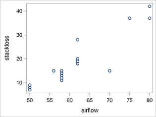
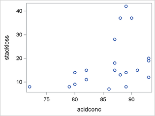
Figure 4 shows the distribution of StackLoss and scatter plots of StackLoss by AirFlow, StackLoss by WaterTemp, and StackLoss by AcidConc. The distribution of StackLoss is bimodal and right-skewed, and it has a noticeable gap between the values of 20 and 28. These characteristics suggest the possibility that the response variable has a mixture distribution.

The relationship between StackLoss and AirFlow appears to be linear. The relationship between StackLoss and WaterTemp is approximately linear, but there is a suggestion of nonlinearity. The relationship between StackLoss and AcidConc might best be described as heteroscedastic. Again, there is a suggestion that the response variable has a mixture distribution because of the apparent clustering of StackLoss as AcidConc increases.

Figure 4: Visual Inspection of the Data

Distribution of Stack Loss	Stack Loss by Air Flow

Stack Loss by Water Temperature	Stackloss by Acid Concentration

Yu and Moyeed (2001) fit the following quantile regression model to these data:

$q_ p = \beta _0(p) + \beta _1(p)*AirFlow + \beta _2(p)*WaterTemp + \beta _3(p)*AcidConc$

The following statements show an efficient way to use the MCMC procedure to request the estimated quantile processes $\hat{\bbeta }(p)$ for the quantile regression parameters. Suppose you span the range of $p$ in increments of 0.05. That is, you want to estimate the $0.05, 0.10, \dots , 0.95$ quantiles; there are 19 quantiles in all. First, you create a new data set that has 19 copies of your original data set. The new data set must be indexed and sorted by $p$ . Second, you use the MCMC procedure’s BY-group processing capabilities to estimate the model parameters for each of the 19 quantiles. The ODS OUTPUT statement saves the “Posterior Summaries” and “Posterior Intervals” tables as SAS data sets. These data sets are used later to produce plots of the quantile processes for each parameter. The DATA= option of the PROC MCMC statement specifies the newly created input data set. The BEGINCNST and ENDCNST statement block, where you previously specified a single value for $p$ , is replaced with a BY statement. < /p>


data by_stackloss;
  set stackloss;
  do p = .05 to .95 by .05;
    output;
  end;
run;


proc sort data=by_stackloss;
  by p;
run;


ods output postsummaries=by_ps postintervals=by_pi;
proc mcmc data=by_stackloss
          seed=73625
          propcov=congra
          ntu=1000
          nmc=30000
          mintune=17;
  by p;
  parms (b0-b3) 0;
  prior b: ~ general(0);
  mu= b0 + b1*airflow + b2*watertemp + b3*acidconc;
  u = stackloss - mu;
  ll = log(p)+log(1-p) - 0.5*(abs(u)+(2*p-1)*u);
  model stackloss ~ general(ll);
run;

The contents of the “Posterior Summaries” and “Posterior Intervals” tables for the whole quantile process are saved in the ODS OUTPUT data sets By_ps and By_pi, respectively. The following statements merge these two data sets, sort the merged data set, and then use the SGPLOT and PRINT procedures to produce quantile process plots and tables for each model parameter:


data process;
  merge by_ps by_pi;
run;


proc sort data=process out=process;
  by parameter p;
run;


proc sgplot data=process(where=(parameter="b0"));
  title "Estimated Parameter by Quantile";
  title2 "With 95% HPD Interval";
  series x=p y=mean / markers legendlabel="Intercept (b0)";
  band x=p lower=hpdlower upper=hpdupper /
       transparency=.5 legendlabel="HPD Interval";
  yaxis label="Intercept (b0)";
  xaxis label="Quantile";
  refline 0 / axis=y;
run;


proc print data=process(where=(parameter="b0")) noobs;
  title "Estimated Parameter b0 by Quantile";
  title2 "with 95% HPD Interval";
  var p mean hpdlower hpdupper;
run;

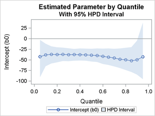
Figure 5 and Output 5 show that the sample means for the intercept, b0, are negative throughout the process. They are increasing up to the 0.15 quantile and are then relatively constant up to the 0.60 quantile. The means then begin a steady decline until the 0.85 quantile, where they begin increasing. The 95% HPD intervals are negative throughout most the process; the exception is the 0.95 quantile, whose 95% HPD interval contains 0.

Figure 5: Quantile Process Plot for b0

Output 5: Quantile Process Table for b0

Estimated Parameter b0 by Quantile

with 95% HPD Interval

p	Mean	HPDLower	HPDUpper
0.05	-42.3985	-90.8604	-3.2819
0.10	-38.1142	-65.1973	-11.9736
0.15	-36.9064	-58.7638	-18.1234
0.20	-37.2556	-55.8252	-20.4854
0.25	-37.2191	-52.7650	-21.1718
0.30	-37.9856	-53.1388	-22.6125
0.35	-37.2883	-52.2435	-24.4803
0.40	-37.6403	-51.7583	-23.0280
0.45	-38.0287	-52.0388	-23.5456
0.50	-38.8226	-54.0858	-24.0051
0.55	-39.9354	-55.3115	-23.0169
0.60	-41.6264	-59.8976	-23.6168
0.65	-43.4826	-62.0332	-23.2145
0.70	-45.5962	-65.6766	-23.9189
0.75	-48.4560	-69.5842	-23.1632
0.80	-49.8484	-73.9430	-21.7130
0.85	-51.8986	-78.5607	-20.1638
0.90	-49.9473	-84.8666	-4.8727
0.95	-42.9003	-95.6122	37.8042

Figure 6 and Output 6 show that the sample means for the parameter b1, the coefficient for AirFlow, are positive throughout the process. The means increase for most of the process, peak at the 0.65 quantile, decrease monotonically until the 0.90 quantile, and then increase slightly. The 95% HPD intervals are all strictly positive except for the 0.05 quantile’s interval, which contains 0.

Figure 6: Quantile Process Plot for b1

Output 6: Quantile Process Table for b1

Estimated Parameter b1 by Quantile

with 95% HPD Interval

p	Mean	HPDLower	HPDUpper
0.05	0.3885	-0.1160	0.8970
0.10	0.4493	0.1007	0.8213
0.15	0.5060	0.1859	0.8358
0.20	0.5871	0.2660	0.8972
0.25	0.6534	0.3645	0.9323
0.30	0.7105	0.4329	0.9787
0.35	0.7515	0.4798	0.9767
0.40	0.7873	0.5527	1.0260
0.45	0.8133	0.5935	1.0535
0.50	0.8315	0.5984	1.0586
0.55	0.8575	0.6314	1.0952
0.60	0.8752	0.6505	1.1113
0.65	0.8847	0.6481	1.1320
0.70	0.8800	0.6196	1.1402
0.75	0.8570	0.5780	1.1169
0.80	0.8391	0.5218	1.1347
0.85	0.7879	0.4486	1.1065
0.90	0.7624	0.3821	1.1625
0.95	0.7639	0.1712	1.4504

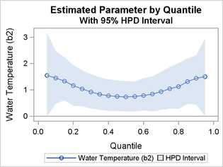
Figure 7 and Output 7 show that the sample means for the parameter b2, the coefficient for WaterTemp, are positive throughout the process. The means decrease monotonically up to the 0.50 quantile and then increase monotonically, forming a quadratic shape. The 95% HPD intervals are all strictly positive.

Figure 7: Quantile Process Plot for b2

Output 7: Quantile Process Table for b2

Estimated Parameter b2 by Quantile

with 95% HPD Interval

p	Mean	HPDLower	HPDUpper
0.05	1.5434	-0.0237	3.1776
0.10	1.4464	0.4691	2.4739
0.15	1.3340	0.5991	2.2340
0.20	1.1584	0.3870	1.9407
0.25	1.0332	0.3694	1.7456
0.30	0.9197	0.2825	1.5866
0.35	0.8305	0.2426	1.4704
0.40	0.7735	0.1924	1.3922
0.45	0.7526	0.1880	1.3552
0.50	0.7331	0.1789	1.3296
0.55	0.7457	0.1715	1.3120
0.60	0.7871	0.2148	1.4364
0.65	0.8367	0.1736	1.5076
0.70	0.9299	0.2258	1.6847
0.75	1.0437	0.2869	1.8634
0.80	1.1216	0.2783	2.0078
0.85	1.3144	0.4507	2.1898
0.90	1.4403	0.4344	2.3049
0.95	1.4978	0.000710	2.9429

Figure 8 and Output 8 show that the sample means for the parameter b3, the coefficient for AcidConc, are relatively constant and close to, but systematically below, 0. The 95% HPD intervals contain 0 throughout the process.

Figure 8: Quantile Process Plot for b3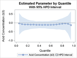

Output 8: Quantile Process Table for b3

Estimated Parameter b3 by Quantile

with 95% HPD Interval

p	Mean	HPDLower	HPDUpper
0.05	-0.0273	-0.6761	0.5518
0.10	-0.0742	-0.5038	0.3504
0.15	-0.0888	-0.4208	0.2613
0.20	-0.0902	-0.3912	0.1849
0.25	-0.0995	-0.3469	0.1370
0.30	-0.0975	-0.3252	0.1201
0.35	-0.1079	-0.3162	0.0850
0.40	-0.1109	-0.3057	0.0971
0.45	-0.1153	-0.3107	0.0875
0.50	-0.1101	-0.3099	0.0961
0.55	-0.1134	-0.3317	0.0889
0.60	-0.1106	-0.3472	0.1124
0.65	-0.1026	-0.3502	0.1337
0.70	-0.0917	-0.3749	0.1417
0.75	-0.0655	-0.3670	0.2100
0.80	-0.0501	-0.3994	0.2571
0.85	-0.0292	-0.4046	0.3260
0.90	-0.0539	-0.6201	0.4144
0.95	-0.1274	-0.9977	0.6559

References

Brownlee, K. A. (1965), Statistical Theory and Methodology in Science and Engineering, New York: John Wiley & Sons.
Isaacs, D., Altman, D. G., Tidmarsh, C. E., Valman, H. B., and Webster, A. D. B. (1983), “Serum Immunoglobulin Concentrations in Preschool Children Measured by Laser Nephelometry: Reference Ranges for IgG, IgA, IgM,” Journal of Clinical Pathology, 36, 1193–1196.
Royston, P. and Altman, D. G. (1994), “Regression Using Fractional Polynomials of Continuous Covariates: Parsimonious Parametric Modelling (with Discussion),” Applied Statistics, 43, 429–467.
Yu, K. and Moyeed, R. A. (2001), “Bayesian Quantile Regression,” Statistics and Probability Letters, 54, 437–447.
Yu, K. and Zhang, J. (2005), “A Three-Parameter Asymmetric Laplace Distribution and Its Extension,” Communications in Statistics—Theory and Methods, 34, 1867–1879.

These sample files and code examples are provided by SAS Institute Inc. "as is" without warranty of any kind, either express or implied, including but not limited to the implied warranties of merchantability and fitness for a particular purpose. Recipients acknowledge and agree that SAS Institute shall not be liable for any damages whatsoever arising out of their use of this material. In addition, SAS Institute will provide no support for the materials contained herein.

data igg;
  input IgG Age;
  Age2=age*age;
  datalines;
      1.5         .5
      2.7         .5
      1.9         .5
        4         .5
      1.9         .5
      4.4         .5
      1.5         .5
      2.2         .5
      1.6         .5
      4.7         .5
      1.6         .5
      1.4         .5
        3         .5
      2.5         .5
        1         .5
      4.3         .5
      4.7         .5
      1.7         .5
      1.9   .5833333
       .9   .5833333
      4.1   .5833333
      2.8   .5833333
      2.2   .5833333
      5.4   .6666667
      8.4   .6666667
        2   .6666667
      5.1   .6666667
      1.5   .6666667
      3.2   .6666667
      7.7        .75
      4.5        .75
      6.6        .75
      4.2        .75
      2.1        .75
      4.2        .75
      3.8        .75
      5.7   .8333333
        3   .8333333
      3.2   .9166667
      5.1   .9166667
      2.1   .9166667
      2.3   .9166667
      3.4   .9166667
      3.9   .9166667
      4.3   .9166667
      5.3   .9166667
      7.2   .9166667
      3.8   .9166667
      5.6   .9166667
      1.5          1
        7          1
      4.6          1
      3.7          1
      4.5          1
      4.5          1
        5          1
      5.5          1
      5.5          1
      3.2          1
      3.2          1
      2.2          1
      2.3          1
      3.8   1.083333
      3.5   1.083333
      5.8   1.083333
        4   1.083333
      2.6   1.083333
      5.1   1.166667
      4.4   1.166667
      3.1   1.166667
        5   1.166667
      1.4   1.166667
      6.7   1.166667
      5.3   1.166667
      1.7   1.166667
      6.6   1.166667
      2.9   1.166667
      6.1       1.25
        4       1.25
      5.5       1.25
      4.7       1.25
      6.1       1.25
        4       1.25
      7.4   1.333333
      4.7   1.333333
      3.9   1.333333
      4.5   1.333333
      5.1   1.416667
      3.4   1.416667
      3.5   1.416667
      3.7        1.5
      5.8        1.5
      4.1        1.5
      9.8        1.5
      2.8        1.5
      5.8   1.583333
        7   1.583333
      3.1   1.583333
      4.2   1.666667
      5.4   1.666667
      5.7   1.666667
      4.4   1.666667
      5.8       1.75
      4.1       1.75
        4       1.75
      5.3       1.75
        5   1.833333
        6   1.833333
      5.7   1.833333
        7   1.833333
      2.5   1.833333
      6.8   1.833333
      6.3   1.916667
      5.3   1.916667
      4.7          2
        7          2
      4.2          2
      5.7          2
      3.4          2
      6.7          2
      4.6          2
      5.6          2
      1.8          2
      3.5          2
      4.3          2
      4.3          2
      5.4          2
      4.9          2
      5.4          2
      5.6          2
      3.8   2.083333
      7.3   2.083333
      3.4   2.083333
      4.4   2.083333
      3.7   2.083333
      3.3   2.083333
      3.5   2.083333
        5   2.083333
      2.7   2.083333
      4.4   2.166667
        8   2.166667
      6.2       2.25
      3.3   2.333333
      5.8   2.333333
      7.5   2.333333
      5.5   2.333333
      5.5        2.5
      6.1        2.5
      4.9   2.583333
      7.2   2.583333
      3.5   2.583333
      5.9   2.666667
      3.2       2.75
      6.1       2.75
      3.7       2.75
      7.3   2.833333
      3.3   2.916667
      1.8   2.916667
     10.4   2.916667
      4.2   2.916667
      4.2          3
      6.1          3
      7.8          3
      4.4          3
        5          3
      5.3          3
      5.6          3
      4.5          3
        6          3
      7.3   3.083333
      4.5   3.083333
      4.7   3.083333
      3.9   3.083333
        4   3.083333
      4.8   3.083333
      3.3   3.083333
      5.7   3.083333
      4.3   3.083333
        7   3.083333
     13.4   3.083333
        4   3.083333
      5.8   3.166667
      6.3   3.166667
      8.8   3.166667
      4.8   3.166667
      5.3       3.25
      4.6       3.25
      6.9       3.25
      5.7   3.333333
      6.5   3.416667
      6.3   3.416667
      6.8   3.416667
      3.9        3.5
      7.8   3.583333
        8   3.583333
      5.4   3.666667
      6.2   3.666667
      6.1   3.833333
      3.9   3.833333
        6   3.833333
      3.5   3.833333
      4.2   3.833333
      3.6   3.833333
      4.3   3.833333
      5.4   3.916667
      5.8          4
      7.5          4
      7.1          4
        6          4
      3.2   4.083333
      6.9   4.083333
      7.9   4.083333
      3.4   4.083333
      9.5   4.166667
      3.8   4.166667
      8.3   4.166667
      6.7   4.166667
      7.1       4.25
      7.8       4.25
      7.2       4.25
      6.6   4.333333
      2.5   4.333333
      2.1   4.333333
        4   4.333333
      3.7   4.333333
      5.6   4.333333
      5.6   4.333333
      4.5   4.416667
      5.9   4.416667
      6.3   4.416667
      4.7   4.416667
        8   4.416667
      4.6   4.416667
        4   4.416667
      1.9   4.416667
        4        4.5
      8.6        4.5
      2.6        4.5
      3.9        4.5
      6.4   4.583333
      7.8   4.583333
      3.8   4.583333
      5.5   4.583333
      7.1   4.583333
     10.2   4.666667
        7   4.666667
      7.4   4.666667
      9.4   4.666667
      6.8   4.666667
      9.1   4.666667
      5.2       4.75
      4.3       4.75
      2.7       4.75
       11       4.75
      9.6   4.833333
     12.6   4.833333
      8.9   4.833333
      3.8   4.916667
      6.1   5.083333
      7.5   5.083333
      7.4   5.083333
     10.9   5.083333
      8.3   5.166667
      8.2   5.166667
      4.7   5.166667
      8.1   5.166667
      9.3   5.166667
      4.4   5.166667
      8.7   5.166667
      9.8       5.25
      7.1       5.25
      8.1       5.25
      7.9       5.25
      8.4   5.333333
      8.2   5.333333
     10.4   5.333333
      9.7   5.333333
      8.1   5.416667
      4.8   5.416667
      4.9        5.5
     12.5        5.5
      3.8        5.5
      8.8        5.5
     10.4   5.583333
      4.7   5.583333
      3.3   5.583333
      5.6   5.583333
      4.6   5.583333
     14.4   5.583333
      9.1   5.666667
      6.3   5.666667
      6.1       5.75
      5.6       5.75
      5.4       5.75
        7   5.833333
      7.6   5.916667
      3.1          6
      6.8          6
;
run;


ods graphics on;
proc sgplot data=igg;
  histogram igg / nbins=50;
run;


proc sgplot data=igg;
  scatter x=Age y=IgG;
run;


proc mcmc data=igg
          seed=5263
          propcov=congra
          ntu=1000
          mintune=10
          nmc=30000;
  begincnst;
    p=0.95;
  endcnst;
  parms (b0-b2) 0;
  prior b: ~ general(0);
  mu= b0 + b1*age + b2*age2;
  u = igg - mu;
  ll = log(p)+log(1-p) - 0.5*(abs(u)+(2*p-1)*u);
  model igg ~ general(ll);
run;


data stackloss;
  input stackloss airflow watertemp acidconc;
  datalines;
42       80         27         89
37       80         27         88
37       75         25         90
28       62         24         87
18       62         22         87
18       62         23         87
19       62         24         93
20       62         24         93
15       58         23         87
14       58         18         80
14       58         18         89
13       58         17         88
11       58         18         82
12       58         19         93
 8       50         18         89
 7       50         18         86
 8       50         19         72
 8       50         19         79
 9       50         20         80
15       56         20         82
15       70         20         91
;
run;


proc sgplot data=stackloss;
  histogram stackloss / nbins=10;
  xaxis label="Stack Loss";
run;


proc sgplot data=stackloss;
  scatter y=stackloss x=airflow;
run;


proc sgplot data=stackloss;
  scatter y=stackloss x=watertemp;
run;


proc sgplot data=stackloss;
  scatter y=stackloss x=acidconc;
run;


data by_stackloss;
  set stackloss;
  do p = .05 to .95 by .05;
    output;
  end;
run;


proc sort data=by_stackloss;
  by p;
run;


ods output postsummaries=by_ps postintervals=by_pi;
proc mcmc data=by_stackloss
          seed=73625
          propcov=congra
          ntu=1000
          nmc=30000
          mintune=17;
  by p;
  parms (b0-b3) 0;
  prior b: ~ general(0);
  mu= b0 + b1*airflow + b2*watertemp + b3*acidconc;
  u = stackloss - mu;
  ll = log(p)+log(1-p) - 0.5*(abs(u)+(2*p-1)*u);
  model stackloss ~ general(ll);
run;


data process;
  merge by_ps by_pi;
run;


proc sort data=process out=process;
  by parameter p;
run;


proc sgplot data=process(where=(parameter="b0"));
  title "Estimated Parameter by Quantile";
  title2 "With 95% HPD Interval";
  series x=p y=mean / markers legendlabel="Intercept (b0)";
  band x=p lower=hpdlower upper=hpdupper /
       transparency=.5 legendlabel="HPD Interval";
  yaxis label="Intercept (b0)";
  xaxis label="Quantile";
  refline 0 / axis=y;
run;


proc print data=process(where=(parameter="b0")) noobs;
  title "Estimated Parameter b0 by Quantile";
  title2 "with 95% HPD Interval";
  var p mean hpdlower hpdupper;
run;


proc sgplot data=process(where=(parameter="b1"));
  title "Estimated Parameter by Quantile";
  title2 "With 95% HPD Interval";
  series x=p y=mean / markers legendlabel="Airflow (b1)";
  band x=p lower=hpdlower upper=hpdupper /
       transparency=.5 legendlabel="HPD Interval";
  yaxis label="Airflow (b1)";
  xaxis label="Quantile";
  refline 0 / axis=y;
run;


proc print data=process(where=(parameter="b1")) noobs;
  title "Estimated Parameter b1 by Quantile";
  title2 "with 95% HPD Interval";
  var p mean hpdlower hpdupper;
run;


proc sgplot data=process(where=(parameter="b2"));
  title "Estimated Parameter by Quantile";
  title2 "With 95% HPD Interval";
  series x=p y=mean / markers legendlabel="Water Temperature (b2)";
  band x=p lower=hpdlower upper=hpdupper /
       transparency=.5 legendlabel="HPD Interval";
  yaxis label="Water Temperature (b2)";
  xaxis label="Quantile";
  refline 0 / axis=y;
run;


proc print data=process(where=(parameter="b2")) noobs;
  title "Estimated Parameter b2 by Quantile";
  title2 "with 95% HPD Interval";
  var p mean hpdlower hpdupper;
run;


proc sgplot data=process(where=(parameter="b3"));
  title "Estimated Parameter by Quantile";
  title2 "With 95% HPD Interval";
  series x=p y=mean / markers legendlabel="Acid Concentration (b3)";
  band x=p lower=hpdlower upper=hpdupper /
       transparency=.5 legendlabel="HPD Interval";
  yaxis label="Acid Concentration (b3)";
  xaxis label="Quantile";
  refline 0 / axis=y;
run;


proc print data=process(where=(parameter="b3")) noobs;
  title "Estimated Parameter b3 by Quantile";
  title2 "with 95% HPD Interval";
  var p mean hpdlower hpdupper;
run;

These sample files and code examples are provided by SAS Institute Inc. "as is" without warranty of any kind, either express or implied, including but not limited to the implied warranties of merchantability and fitness for a particular purpose. Recipients acknowledge and agree that SAS Institute shall not be liable for any damages whatsoever arising out of their use of this material. In addition, SAS Institute will provide no support for the materials contained herein.

This sample demonstrates how to perform Bayesian quantile regression by using SAS/STAT software’s MCMC procedure.

Type:	Sample
Topic:	Analytics ==> Bayesian Analysis SAS Reference ==> Procedures ==> MCMC

Date Modified:	2017-01-12 15:26:05
Date Created:	2016-10-25 10:24:10

Operating System and Release Information

Product Family	Product	Host	SAS Release
Product Family	Product	Host	Starting	Ending
SAS System	SAS/STAT	z/OS
		z/OS 64-bit
		OpenVMS VAX
		Microsoft® Windows® for 64-Bit Itanium-based Systems
		Microsoft Windows Server 2003 Datacenter 64-bit Edition
		Microsoft Windows Server 2003 Enterprise 64-bit Edition
		Microsoft Windows XP 64-bit Edition
		Microsoft® Windows® for x64
		OS/2
		Microsoft Windows 8 Enterprise 32-bit
		Microsoft Windows 8 Enterprise x64
		Microsoft Windows 8 Pro 32-bit
		Microsoft Windows 8 Pro x64
		Microsoft Windows 8.1 Enterprise 32-bit
		Microsoft Windows 8.1 Enterprise x64
		Microsoft Windows 8.1 Pro 32-bit
		Microsoft Windows 8.1 Pro x64
		Microsoft Windows 10
		Microsoft Windows 95/98
		Microsoft Windows 2000 Advanced Server
		Microsoft Windows 2000 Datacenter Server
		Microsoft Windows 2000 Server
		Microsoft Windows 2000 Professional
		Microsoft Windows NT Workstation
		Microsoft Windows Server 2003 Datacenter Edition
		Microsoft Windows Server 2003 Enterprise Edition
		Microsoft Windows Server 2003 Standard Edition
		Microsoft Windows Server 2003 for x64
		Microsoft Windows Server 2008
		Microsoft Windows Server 2008 R2
		Microsoft Windows Server 2008 for x64
		Microsoft Windows Server 2012 Datacenter
		Microsoft Windows Server 2012 R2 Datacenter
		Microsoft Windows Server 2012 R2 Std
		Microsoft Windows Server 2012 Std
		Microsoft Windows XP Professional
		Windows 7 Enterprise 32 bit
		Windows 7 Enterprise x64
		Windows 7 Home Premium 32 bit
		Windows 7 Home Premium x64
		Windows 7 Professional 32 bit
		Windows 7 Professional x64
		Windows 7 Ultimate 32 bit
		Windows 7 Ultimate x64
		Windows Millennium Edition (Me)
		Windows Vista
		Windows Vista for x64
		64-bit Enabled AIX
		64-bit Enabled HP-UX
		64-bit Enabled Solaris
		ABI+ for Intel Architecture
		AIX
		HP-UX
		HP-UX IPF
		IRIX
		Linux
		Linux for x64
		Linux on Itanium
		OpenVMS Alpha
		OpenVMS on HP Integrity
		Solaris
		Solaris for x64
		Tru64 UNIX

Support

Sample 59222: Bayesian Quantile Regression

Overview

Analysis

Fitting a Single Quantile Regression Function

Fitting a Quantile Process

References

Operating System and Release Information