Sample 59778: Calculating Elasticities in an Almost Ideal Demand System
 |  |  |  |
Overview
Economists are often interested in price and income elasticities. Price elasticity is defined as the percentage change in quantity demanded for some good with respect to a one percent change in the price of the good (own price elasticity) or of another good (cross price elasticity). Mathematically,
where ![]() is the cross price
elasticity for
is the cross price
elasticity for ![]() , own price
elasticity for i=j, pi is
the price on the ith good, and qi is the quantity demanded for the ith good. Price elasticity greater than 1 is called price elastic, and price elasticity
smaller than 1 is called price inelastic. A given percentage increase in the price of an elastic good will reduce the
quantity demanded for the good by a higher percentage than for an inelastic good.
, own price
elasticity for i=j, pi is
the price on the ith good, and qi is the quantity demanded for the ith good. Price elasticity greater than 1 is called price elastic, and price elasticity
smaller than 1 is called price inelastic. A given percentage increase in the price of an elastic good will reduce the
quantity demanded for the good by a higher percentage than for an inelastic good.
Income elasticity is defined as the percentage change in quantity demanded with respect to a one percent change in income.
where x is total income.
Price elasticities can either be derived from the Marshallian demand equation or the Hicksian demand equation. The Marshallian demand equation is obtained from maximizing utility subject to the budget constraint, while the Hicksian demand equation is derived from solving the dual problem of expenditure minimization at a certain utility level. Elasticities derived from Marshallian demand are called Marshallian or uncompensated elasticities, and elasticities derived from Hicksian demand are called Hicksian or compensated elasticities. Marshallian elasticities can be transformed into Hicksian elasticities through the Slutsky equation:
where ![]() represents Hicksian
elasticity,
represents Hicksian
elasticity, ![]() represents
Marshallian elasticity, wj is the budget share on good j, and ei is the income elasticity for
good i. More detailed discussions on the Marshallian and the Hicksian demand relations
and the Slutsky equation can be found in many standard economics textbooks; see Nicholson (1992) and Gravelle and Rees
(1992).
represents
Marshallian elasticity, wj is the budget share on good j, and ei is the income elasticity for
good i. More detailed discussions on the Marshallian and the Hicksian demand relations
and the Slutsky equation can be found in many standard economics textbooks; see Nicholson (1992) and Gravelle and Rees
(1992).
Analysis
In this example, you calculate the Marshallian and the Hicksian price elasticities and the income elasticity for the Almost Ideal Demand System (AIDS) model described in the example "Estimating an Almost Ideal Demand System Model." The model is as follows:
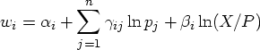
where wi is the share associated with the ith good, ![]() is the slope coefficient associated with the j th good in the
i th share equation, and pj is
the price on the j th good. X is the total expenditure on the system of goods, and P is
the price index.
is the slope coefficient associated with the j th good in the
i th share equation, and pj is
the price on the j th good. X is the total expenditure on the system of goods, and P is
the price index.
The AIDS model implies that the Marshallian price elasticity for good i with respect to good j is
where
Income elasticity is given by
If you are interested in elasticities at a specific point, an ESTIMATE statement can be used in the MODEL procedure to obtain estimates and standard errors of the elasticity at that point. For example, if you want to calculate own price elasticity for beef, and you know both the budget share for beef, say, 0.5, and ln(X/P), say, 9.0, then you can use an ESTIMATE statement in the MODEL procedure as follows (see "Estimating an Almost Ideal Demand System Model" for more code in the MODEL statement):
   data aids_;
     input year qtr pop b_q p_q c_q t_q b_p p_p c_p t_p cpi pc_exp;


   ... more datalines ...

   ;
   run;
   /* Full Nonlinear AIDS Model */
   proc model data=aids;


      w_b = ab + gbb*lpb + gbp*lpp + gbc*lpc + gbt*lpt + bb*(lx-p) + abco1*co1
               + absi1*si1 + ab_t*t ;
      w_p = ap + gbp*lpb + gpp*lpp + gpc*lpc + gpt*lpt + bp*(lx-p) + apco1*co1
               + apsi1*si1 + ap_t*t ;
      w_c = ac + gbc*lpb + gpc*lpp + gcc*lpc + gct*lpt + bc*(lx-p) + acco1*co1
               + acsi1*si1 + ac_t*t ;

      fit w_b w_p w_c / itsur nestit outs=rest outest=fin2 converge = .00001
                        maxit = 1000 ;
      parms ab bb gbb gbp gbc gbt abco1 absi1 ab_t
            ap bp     gpp gpc gpt apco1 apsi1 ap_t
            ac bc         gcc gct acco1 acsi1 ac_t
            at                gtt ;
      estimate 'elasticity beef' (gbb - bb*(.5 - bb*9.0))/.5 - 1;

   run;
   quit;
This will yield the estimate for the elasticity when the budget share for beef is 0.5, and ln(X/P) = 9.0. The output is shown below.
|
The MODEL Procedure
|
||||||||||||||||||
The estimated own price elasticity for beef suggests that increasing the price for beef by 1% will reduce the demand for beef by 0.94%. Such information will be useful for setting prices. The ESTIMATE statement also provides standard error estimates.
If you are not interested in standard errors on the elasticities, and you want to compute all own price and cross price elasticities for the system, it is more convenient to do it in IML as shown below. Recall that the parameters estimated in the nonlinear AIDS model are in the data set fin2. The variables not needed in the calculation are eliminated in the following data step so it is easier to read the data set into IML.
To calculate elasticities for the nonlinear AIDS model, you first need to read in the estimated parameters from the output data set fin2:
proc iml;
  use fin2;
  read all var {gbb gbp gbc gbt gpp gpc gpt gcc gct gtt} ;
  read all var {bb bp bc ab ap ac at} ;

  close fin2;
Note that the elasticities have meanings only at a specific data point. In the current example, you calculate the elasticities at the mean point of the data. The following example illustrates the nonlinear AIDS case.
  /* recall meanw contains the means of the variables */
  use meanw;

  /* read in the mean shares */
  read all var {w_b w_p w_c w_t} ;
  /* read in the mean price and expenditure */
  read all var {bm pm cm tm x } ;

  lpb = log(bm);
  lpp = log(pm);
  lpc = log(cm);
  lpt = log(tm);
  lx=log(x);

  close meanw;
To calculate the elasticity matrix with own price elasticity as diagonal elements and cross price elasticities as off diagonal elements, you can express the parameters in matrix form and use matrix manipulation in the calculation.
  /* Budget share vector */
  w = w_b//w_p//w_c//w_t;

  /* gamma(i,j) matrix */
  gij = (gbb||gbp||gbc||gbt)//
        (gbp||gpp||gpc||gpt)//
        (gbc||gpc||gcc||gct)//
        (gbt||gpt||gct||gtt);

  /* turkey parameter based on sum-to-one constraint */
  bt= 0-bb-bp-bc;

  a=ab//ap//ac//at;  /* alpha(i) vector */
  b=bb//bp//bc//bt;  /* beta(i) vector  */
You then specify the nonlinear price index as described in the example "Estimating an Almost Ideal Demand System Model":
  a0=0;
  p = a0 + ab*lpb + ap*lpp + ac*lpc + at*lpt +
  .5*(gbb*lpb*lpb + gbp*lpb*lpp + gbc*lpb*lpc + gbt*lpb*lpt +
      gbp*lpp*lpb + gpp*lpp*lpp + gpc*lpp*lpc + gpt*lpp*lpt +
      gbc*lpc*lpb + gpc*lpc*lpp + gcc*lpc*lpc + gct*lpc*lpt +
      gbt*lpt*lpb + gpt*lpt*lpp + gct*lpt*lpc + gtt*lpt*lpt );
Now you calculate each element of the elasticity matrix:
  nk=ncol(gij);

  mi = -1#I(nk);

  ff2 = j(nk,nk,0);   /* Initialize Marshallian elasticity matrix */
  fic2 = j(nk,nk,0);  /* Initialize Hicksian elasticity matrix */
  fi2 = j(nk,1,0);    /* Income elasticity vector */


  /* prepare for plotting the elasticity matrices*/

  /* initialize index vectors for the X- and Y-axis */
  x = j(nk*nk,1,0);
  y = j(nk*nk,1,0);

  /* initialize vector to store elasticity matrices */
  Helast = j(nk*nk,1,0);
  Melast = j(nk*nk,1,0);

  i=1;
  do i=1 to nk;
    fi2[i,1] = 1 + b[i,]/w[i,];
    j=1;
      do j=1 to nk;
        ff2[i,j] = mi[i,j] + (gij[i,j] - b[i,]#(w[j,]-b[j,]#(lx-p)))/w[i,];
        fic2[i,j] = ff2[i,j] + w[j,]#fi2[i,];
        x[(i-1)*nk+j,1] = i ;
        y[(i-1)*nk+j,1] = j ;
        Melast[(i-1)*nk+j,1] = ff2[i,j] ;
        Helast[(i-1)*nk+j,1] = fic2[i,j] ;
      end;
  end;


  /*create data set for plotting*/
  create plotdata var{x y Melast Helast} ;
  append;
  close plotdata;
  run;
  quit;
The calculated Marshallian elasticity matrix for the nonlinear AIDS model is given below:
The results show that all own price elasticities are negative, and all of the elasticities are less than 1 in absolute value, meaning that all goods are inelastic.
The income elasticities are reported below:
|
|
The results show that turkey consumption is the most sensitive to income changes, while chicken consumption is the least sensitive to income changes.
Finally, the Hicksian elasticity matrix is given below:
|
||||||||||||||||||||||||||||||
The own price Hicksian elasticities are also negative for all four goods as expected.
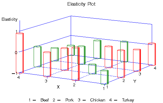
The following statements illustrate plotting the Hicksian elasticity in three dimensions.
   proc g3d data = plotdata;

      scatter x*y=Helast

         / grid
           shape='pillar'
           color=colorval
           caxis=blue
           rotate=60
           size=2.5
           yticknum=4
           xticknum=4
           zticknum=3
           zmin=-1
           zmax=1;

   run;
   quit;
The Hicksian elasticity matrix is plotted in the figure shown below. The red bar indicates positive elasticity, while the green bar indicates negative elasticity.
|
Figure 1: Hicksian Elasticity
Acknowledgment
The SAS program used in this example is based on code provided by Dr. Barry Goodwin.
References
Gravelle, H., and Rees, R. (1992), Microeconomics, New York: Longman Publishing.
Nicholson, W. (1992), Microeconomic Theory: Basic Principles and Extensions, Fifth Edition, Fort Worth: Dryden Press.
SAS Institute Inc. (1999), SAS/ETS User's Guide, Version 8, Cary, NC: SAS Institute Inc.
These sample files and code examples are provided by SAS Institute Inc. "as is" without warranty of any kind, either express or implied, including but not limited to the implied warranties of merchantability and fitness for a particular purpose. Recipients acknowledge and agree that SAS Institute shall not be liable for any damages whatsoever arising out of their use of this material. In addition, SAS Institute will provide no support for the materials contained herein.
   /*------------------------------------------------------------------
     Example: Calculating Elasticities in an Almost Ideal Demand System
     Requires: SAS/ETS
     Version: 9.0
     -------------------------------------------------------------------*/


data aids_;
  input year qtr pop b_q p_q c_q t_q b_p p_p c_p t_p cpi pc_exp;
  datalines;
1970 1 204.082 21.0583 12.9527 9.5757      0.8674     99.1333      85.8      42.17     56.3      38        776.2811
1970 2 204.719 20.8497 13.1503 10.6764     0.9824     100.5333     84        41        58.1      38.63     786.2015
1970 3 205.418 21.5885 13.6835 10.5298     2.1212     101.3        82.9      40.4      56.23     39.07     798.1306
1970 4 206.131 21.1168 15.9879 9.7563      4.1365     98.8         74.8      39.43     55.87     39.6      803.4939
1971 1 206.762 20.5807 15.3589 9.7865      0.9762     101.9        72.7      40.17     54.6      39.9      824.2589
1971 2 207.361 20.9973 14.8311 10.308      1.2525     106.7333     72.3      41.27     53.73     40.33     838.7546
1971 3 207.998 21.7098 14.9318 10.503      2.061      107.5        74.9      42.27     56.3      40.77     850.9718
1971 4 208.648 20.6377 15.4272 9.9795      4.0973     108.8333     75.5      40.5      55.63     40.97     867.8513
1972 1 209.137 20.5323 14.4696 10.3073     1.1039     116.9667     83.1      41.37     56.7      41.27     886.6219
1972 2 209.635 21.4144 13.6081 11.0482     1.3421     115          84        40.67     56.67     41.6      906.218
1972 3 210.177 21.5884 12.7471 10.5941     2.1463     118.2667     90.5      42        56.03     42        925.6506
1972 4 210.739 21.742  13.8372 10.0881     4.3869     116.3333     92.3      41.47     56.57     42.4      952.721
1973 1 211.187 20.593  12.6767 9.8371      1.1771     132.9333     103.2     49.93     58.6      42.93     980.0556
1973 2 211.662 19.3625 12.2869 10.3858     1.2922     139.9        108.5     58.33     69.5      43.9      995.8117
1973 3 212.191 19.7379 11.0802 10.1065     2.1009     146.2667     128.2     74.9      79.68     44.87     1015.479
1973 4 212.71  20.8158 12.7018 9.8959      3.8408     139.5667     122.2     55.33     90.27     45.9      1030.984
1974 1 213.143 20.6926 13.0753 10.011      1.1952     150.0333     121.4     58.47     81.63     47.2      1050.236
1974 2 213.6   21.0231 13.5908 10.6635     1.5227     139.3333     104.6     53        71.07     48.53     1080.995
1974 3 214.144 21.7508 12.8968 10.3135     1.9605     146.2333     113.2     54.1      66.43     50        1110.701
1974 4 214.704 22.1169 13.1451 9.1444      3.9912     139.6667     117       58.27     71.43     51.5      1116.889
1975 1 215.132 22.0991 11.8074 9.2631      1.0724     134.8333     120.8     58.9      72.13     52.43     1143.951
1975 2 215.646 21.0304 11.0085 10.1645     1.3916     152.6333     129.8     58.97     70.83     53.23     1175.193
1975 3 216.294 22.2717 9.6583  10.2047     1.8937     163.2        157.4     68.93     73.87     54.37     1210.39
1975 4 216.851 22.7502 10.4302 9.7381      3.9068     158.1667     161.8     66.3      78.27     55.23     1240.483
1976 1 217.315 23.8753 10.939  10.3294     1.145      148.7        149.4     61.93     78.1      55.77     1278.214
1976 2 217.773 22.8964 10.3597 10.9598     1.5151     148.2        146.3     60.7      77        56.47     1298.485
1976 3 218.337 24.4652 11.0404 11.031      2.0091     142.8        145.1     60.9      76.87     57.37     1329.141
1976 4 218.92  23.1085 13.1403 10.1654     4.2247     142.9333     126.6     55.13     78.23     58.03     1365.91
1977 1 219.424 22.9976 11.9593 10.3395     1.2198     142.1667     127.2     58.27     76.07     59.03     1403.219
1977 2 219.953 22.6131 11.4488 11.2841     1.3872     143.9333     128.8     60.8      74.1      60.33     1432.468
1977 3 220.573 23.4054 11.2324 11.1785     2.109      146.5        138.6     61.9      76.83     61.2      1464.254
1977 4 221.206 22.7401 12.3959 10.4996     4.0197     150.8        135.7     59.3      80.42     61.87     1503.011
1978 1 221.711 22.0441 11.6947 10.8966     1.2211     160          144.9     61.4      74.53     62.93     1533.306
1978 2 222.278 21.7602 11.4791 11.8033     1.589      182.5333     150.7     66.93     79.6      64.53     1595.978
1978 3 222.929 21.6064 11.4611 11.6097     2.0336     186.2        153.1     70.5      84.37     66.07     1628.433
1978 4 223.574 21.8814 12.3615 11.1396     3.88       186.4333     158.8     67.07     87.73     67.4      1666.79
1979 1 224.144 20.5086 12.1608 11.4686     1.3533     211.7        165.1     69.6      90.33     69.07     1708.165
1979 2 224.738 19.0408 13.1374 12.6605     1.7558     231.5        156.8     70.33     91.03     71.47     1743.034
1979 3 225.421 19.1457 13.5239 12.582      2.1241     222.7        146       65.93     89.83     73.83     1796.749
1979 4 226.135 19.3989 14.8575 11.6184     4.0155     223.8333     142.1     64.87     88.17     75.93     1842.373
1980 1 226.753 18.947  14.5643 12.1178     1.7761     231.1667     141.7     67.57     92.77     78.93     1891.931
1980 2 227.387 18.898  14.8637 12.6824     1.9508     227.5        132.5     63.53     90.2      81.83     1890.284
1980 3 228.07  19.2127 13.5274 11.7869     2.5774     237.5333     152.6     75.07     93.63     83.33     1947.981
1980 4 228.696 19.4988 14.3512 11.4689     3.9459     238.1667     163.2     77.27     98.17     85.53     2010.534
1981 1 229.148 19.3429 14.0974 12.0277     1.6042     233.5        157.3     75.43     98.13     87.8      2065.373
1981 2 229.668 18.9816 13.4164 12.6866     1.9006     230.7        153.1     71.9      98.47     89.83     2097.266
1981 3 230.3   19.6459 13.0621 12.8079     2.4992     239.0333     166.6     74.9      101.83    92.37     2139.062
1981 4 230.906 19.2868 14.0918 11.9454     4.5618     235.4333     167.9     70.47     92.97     93.7      2150.663
1982 1 231.392 18.8193 12.7405 11.9425     1.7318     233.3        169.4     71.77     92.47     94.47     2185.69
1982 2 231.901 18.7968 12.2607 12.834      2.0328     242.9667     179.2     72.13     91.3      95.9      2208.706
1982 3 232.496 19.9882 11.5797 12.9951     2.5874     244.0333     195.7     72.33     95.47     97.7      2251.334
1982 4 233.077 19.4242 12.5368 11.8858     4.2141     233.1333     198       69.2      92.9      97.93     2307.933
1983 1 233.543 19.2252 12.114  12.4026     2.0296     233.8667     193.6     69.53     92.07     97.87     2342.609
1983 2 234.02  19.3361 12.7472 13.129      2.1634     240.9333     181       68.73     92.57     99.1      2414.324
1983 3 234.601 20.4952 12.8496 12.5883     2.4668     234.3667     175       74.43     92.7      100.27    2471.643
1983 4 235.157 19.5995 14.0587 11.6903     4.3635     227.1667     169.1     77.17     91.33     101.17    2527.997
1984 1 235.601 19.3191 12.8106 12.3375     1.9057     238.4667     170.9     85.13     94.33     102.3     2575.435
1984 2 236.077 19.3744 12.6312 13.3105     2.155      238          168.7     82.4      97.2      103.4     2627.75
1984 3 236.655 19.9738 12.3802 13.1955     2.5966     232.2        173.5     80.23     101.77    104.53    2659.045
1984 4 237.238 19.7597 13.6804 12.6693     4.3788     233.2333     172.7     76.27     102.37    105.3     2706.149
1985 1 237.667 19.0586 12.7537 12.7081     1.9896     234.9        175       77.13     107.23    105.97    2769.526
1985 2 238.172 20.0757 12.855  13.7851     2.1634     230.4333     167.8     75.67     103.43    107.27    2815.297
1985 3 238.789 20.8175 12.8035 13.5748     2.7299     222.7333     170.4     75.73     105.23    108.03    2878.907
1985 4 239.392 19.2488 13.4707 13.0119     4.7012     226.4333     172.4     76.77     104.93    109       2909.036
1986 1 239.858 19.0212 12.4462 13.0699     2.3152     229.2667     177.4     76.8      106.3     109.23    2944.555
1986 2 240.365 20.1607 12.3281 14.1113     2.3758     222.9        173.2     77.2      103.3     109       2971.522
1986 3 240.961 20.7108 11.5663 13.813      3.0149     225.6333     200.3     91.9      109       109.8     3038.459
1986 4 241.544 18.9416 12.6462 13.2814     5.1658     229.3        204.1     88.1      107.7     110.4     3073.98
1987 1 242.005 18.2746 12.2342 14.0183     2.5318     230.6        195.7     81.9      103.27    111.63    3110.893
1987 2 242.516 18.5266 11.7023 14.5088     2.8807     239.1        194       78.17     102.77    113.1     3176.601
1987 3 243.118 19.175  11.7285 14.5456     3.4995     242.1667     206.9     77.77     104.73    114.4     3234.547
1987 4 243.724 17.8807 13.513  14.2982     5.8184     241.6667     200.7     76.1      93.97     115.37    3264.861
1988 1 244.205 18.1678 12.8332 14.3959     3.035      241.7333     194.6     74.6      92.33     116.07    3337.155
1988 2 244.708 18.4639 12.5507 14.7447     3.4076     250.1        195.5     80.8      91.73     117.53    3391.287
1988 3 245.352 18.7622 12.9249 14.2711     3.7854     254.5333     196.7     95.77     98.7      119.1     3451.164
1988 4 245.97  17.2552 14.1567 14.0575     5.4503     255          189.4     90.3      100.1     120.33    3516.791
1989 1 246.454 16.9765 12.8213 14.3563     3.1189     260.7        190.5     90.57     97.27     121.67    3562.328
1989 2 247.01  17.5192 13.0187 15.0116     3.2763     266.9667     188.9     95.83     99.9      123.67    3616.149
1989 3 247.695 17.5975 12.6332 15.0852     4.1933     268.0333     194.6     95.33     103.57    124.67    3660.659
1989 4 248.38  17.2416 13.5038 14.8018     6.0078     266.9333     199.8     89.07     96.8      125.87    3699.07
1990 1 248.92  16.5516 12.5572 14.9451     3.5354     272.6333     207.6     90.2      98.87     128.03    3771.099
1990 2 249.562 17.3763 11.8816 15.4012     3.6762     281.2        220.5     90.9      98.9      129.33    3812.888
1990 3 250.301 17.4207 12.1079 15.5829     4.2115     280.3667     235.5     91.2      101.83    131.57    3866.944
1990 4 251.04  16.4315 13.216  15.5973     6.1275     289.8667     236       87.37     97.57     133.7     3877.278
1991 1 251.649 15.9842 12.2575 15.1466     3.6626     294.2667     227.6     89.6      99.47     134.8     3879.014
1991 2 252.299 17.0449 12.0445 16.4942     3.9074     295.2        225.6     88.2      101.03    135.6     3922.536
1991 3 253.041 17.5591 12.2515 16.5271     4.0353     284.6333     227       87.7      103.1     136.67    3950.158
1991 4 253.756 16.2093 13.8041 15.8341     6.2823     279.2        216.4     86.63     95.67     137.7     3964.044
1992 1 254.337 16.3952 13.1929 16.8084     3.4475     282.2667     210.4     86.2      95.37     138.67    4052.8
1992 2 255.04  16.9538 12.697  17.1634     3.7342     286.8333     207.3     85.87     98.47     139.8     4089.064
1992 3 255.832 17.227  13.2128 17.3147     4.2        282.6667     211.8     88.03     100.1     140.9     4129.378
1992 4 256.561 15.9093 13.9768 16.4821     6.4864     286.6667     208.5     87.63     93.97     141.9     4207.877
1993 1 257.157 15.8915 13.018  17.3378     3.5527     292.1333     205.9     87.5      99.07     143.1     4229.517
1993 2 257.785 16.2058 12.6251 17.9871     3.7316     300.4        205.5     88.43     101.37    144.2     4287.787
1993 3 258.511 17.043  12.8477 17.9543     3.9801     292          211.8     89.43     102.43    144.77    4340.434
1993 4 259.177 15.9513 13.8657 16.9636     6.4533     289.2333     213.2     90.7      97.5      145.77    4397.293
1994 1 259.65  16.2494 12.5018 17.516      3.5479     286.6667     212.5     89.27     98.5      146.7     4442.326
1994 2 260.261 16.8868 12.9018 18.0614     3.7688     286.1667     210.4     90.63     98.83     147.63    4493.086
1994 3 260.948 17.3775 13.1741 18.6015     4.414      279.5        210.5     90.87     102.73    148.93    4553.589
1994 4 261.59  16.4723 14.4918 17.3363     6.1044     279.1667     204.8     89.6      100.07    149.63    4607.696
1995 1 262.123 16.3097 13.1044 17.9111     3.5628     283.8667     202.7     90.23     99.77     150.87    4643.431
1995 2 262.707 17.0895 12.9167 18.5493     3.9053     283.1        201.2     90.33     102.9     152.2     4704.585
1995 3 263.396 17.647  12.6978 17.343      4.1648     285.1        206.9     92.2      106.53    152.87    4750.642
1995 4 264.055 16.3476 13.7183 17.0398     6.173      285.2667     213.5     93.9      100.27    153.6     4789.163
1996 1 264.535 17.0783 12.6109 18.2436     3.7235     278.7        218.3     93.8      105.03    155       4848.611
1996 2 265.13  17.6763 11.5758 18.6502     3.9        277.4        227.4     95.47     103.27    156.53    4920.237
1996 3 265.836 17.1606 12.0383 18.5709     4.6382     279.8        243.8     98.93     106.5     157.37    4950.138
1996 4 266.515 16.2764 12.8608 17.486      6.206      285.0333     245.4     100.87    102.5     158.5     5007.138
1997 1 267.032 16.2921 11.7752 17.559      3.4603     278.8        244.4     101.1     105.9     159.57    5084.419
1997 2 267.668 17.2994 11.5617 18.7398     3.9826     278.9667     243.1     100.07    105.17    160.2     5105.495
1997 3 268.402 17.0513 12.0187 18.4364     4.1989     281.0667     248.1     99.5      108.5     160.83    5187.275
1997 4 269.085 16.2354 13.3464 17.635      5.9572     279.3        244.4     100.1     100.67    161.47    5231.897
1998 1 269.583 16.6884 12.7173 17.464      3.9209     273.4667     245.6     102.03    101.03    161.9     5299.584
1998 2 270.216 17.1985 12.3142 18.1367     3.9191     278.1        239.8     102.57    97.33     162.77    5381.075
1998 3 270.949 17.5085 13.0799 18.5167     4.1742     277.3667     244.9     105.53    102.8     163.4     5434.243
1998 4 271.633 16.6475 14.384  18.7589     6.0081     279.5333     240.4     107.33    97.1      163.97    5497.951
1999 1 272.136 16.6785 13.5476 19.5127     3.84       278          235.8     106.43    98.47     164.6     5595.374
1999 2 272.774 17.7635 13.055  19.9553     3.831      284.7667     238.4     104.13    97.2      166.2     5683.103
1999 3 273.52  17.6689 13.218  19.2361     4.3288     289.2333     246.4     105.6     102.77    167.23    5761.655
;
run;


data aids;
  set aids_;
  if year < 1975 then delete;
  t = _n_ ;
  co1 = cos(1/2*3.14159*t);
  co2 = cos(2/2*3.14159*t);

  si1 = sin(1/2*3.14159*t);
  si2 = sin(2/2*3.14159*t);

  x = b_p*b_q + p_p*p_q + c_p*c_q + t_p*t_q;

  w_b = b_p*b_q/x;
  w_p = p_p*p_q/x;
  w_c = c_p*c_q/x;
  w_t = t_p*t_q/x;
run;


proc means data=aids noprint;
   var b_p p_p c_p t_p;
   output out=pm mean=b_m p_m c_m t_m;
run;


data aids ;
  if _n_ = 1 then set pm ;
  set aids ;

  pb_ = (b_p/b_m);
  pp_ = (p_p/p_m);
  pc_ = (c_p/c_m);
  pt_ = (t_p/t_m);

  lpb = log(pb_);
  lpp = log(pp_);
  lpc = log(pc_);
  lpt = log(pt_);

  lx = log(x);

  lp0 = sum(w_b*lpb + w_p*lpp + w_c*lpc + w_t*lpt);

  lxp = lx-lp0;
run;


proc means data=aids noprint;
   var w_b w_p w_c w_t pb_ pp_ pc_ pt_ x lp0;
   output out=meanw mean= w_b w_p w_c w_t bm pm cm tm x lp0;
run;


/* Linear Approximate AIDS (LA-AIDS) Model*/
ods html;
proc model data = aids;

  gbt = 0-gbb-gbp-gbc;
  gpt = 0-gbp-gpp-gpc;
  gct = 0-gbc-gpc-gcc;

  w_b = ab + gbb*lpb + gbp*lpp + gbc*lpc + gbt*lpt + bb*lxp;
  w_p = ap + gbp*lpb + gpp*lpp + gpc*lpc + gpt*lpt + bp*lxp;
  w_c = ac + gbc*lpb + gpc*lpp + gcc*lpc + gct*lpt + bc*lxp;

  fit w_b w_p w_c / itsur nestit outest=fin0
                    converge = 0.00001 maxit = 1000 ;
  parms ab bb gbb gbp gbc
        ap bp     gpp gpc
        ac bc         gcc ;
  estimate 'elasticity beef' (gbb - bb*(.5 - bb*9.0))/.5 - 1 ;

run;
quit;


/* Full Nonlinear AIDS Model */
ods html;
proc model data=aids;

  restrict gbb + gbp + gbc + gbt = 0 ,
           gbp + gpp + gpc + gpt = 0 ,
           gbc + gpc + gcc + gct = 0 ,
           gbt + gpt + gct + gtt = 0 ,
           ab + ap + ac + at = 1 ;

  a0 = 0;
  p = a0 + ab*lpb + ap*lpp + ac*lpc + at*lpt +
       .5*(gbb*lpb*lpb + gbp*lpb*lpp + gbc*lpb*lpc + gbt*lpb*lpt +
        gbp*lpp*lpb + gpp*lpp*lpp + gpc*lpp*lpc + gpt*lpp*lpt +
        gbc*lpc*lpb + gpc*lpc*lpp + gcc*lpc*lpc + gct*lpc*lpt +
        gbt*lpt*lpb + gpt*lpt*lpp + gct*lpt*lpc + gtt*lpt*lpt );

  w_b = ab + gbb*lpb + gbp*lpp + gbc*lpc + gbt*lpt + bb*(lx-p) + abco1*co1
           + absi1*si1 + ab_t*t ;
  w_p = ap + gbp*lpb + gpp*lpp + gpc*lpc + gpt*lpt + bp*(lx-p) + apco1*co1
           + apsi1*si1 + ap_t*t ;
  w_c = ac + gbc*lpb + gpc*lpp + gcc*lpc + gct*lpt + bc*(lx-p) + acco1*co1
           + acsi1*si1 + ac_t*t ;

  fit w_b w_p w_c / itsur nestit outs=rest outest=fin2 converge = .00001
                    maxit = 1000 ;
  parms ab bb gbb gbp gbc gbt abco1 absi1 ab_t
        ap bp     gpp gpc gpt apco1 apsi1 ap_t
        ac bc         gcc gct acco1 acsi1 ac_t
        at                gtt ;
  estimate 'elasticity beef' (gbb - bb*(.5 - bb*9.0))/.5 - 1;

run;
quit;


data fin2;
  set fin2;
  drop _name_ _type_ _status_ _nused_;
run;


/* Elasticities  for Nonlinear AIDS Model */
proc iml;
  use fin2;
  read all var {gbb gbp gbc gbt gpp gpc gpt gcc gct gtt} ;
  read all var {bb bp bc ab ap ac at} ;

  close fin2;

  /* recall meanw contains the means of the variables */
  use meanw;

  /* read in the mean shares */
  read all var {w_b w_p w_c w_t} ;
  /* read in the mean price and expenditure */
  read all var {bm pm cm tm x } ;

  lpb = log(bm);
  lpp = log(pm);
  lpc = log(cm);
  lpt = log(tm);
  lx=log(x);

  close meanw;

  /* To calculate the elasticity matrix with own price elasticity
     as diagonal elements and cross price elasticities as off diagonal elements,
  you can express the parameters in matrix form and use matrix manipulation
  in the calculation*/

  /* Budget share vector */
  w = w_b//w_p//w_c//w_t;

  /* gamma(i,j) matrix */
  gij = (gbb||gbp||gbc||gbt)//
        (gbp||gpp||gpc||gpt)//
        (gbc||gpc||gcc||gct)//
        (gbt||gpt||gct||gtt);

  /* turkey parameter based on sum-to-one constraint */
  bt= 0-bb-bp-bc;

  a=ab//ap//ac//at;  /* alpha(i) vector */
  b=bb//bp//bc//bt;  /* beta(i) vector  */


  /* Then specify the nonlinear price index */
  a0=0;
  p = a0 + ab*lpb + ap*lpp + ac*lpc + at*lpt +
  .5*(gbb*lpb*lpb + gbp*lpb*lpp + gbc*lpb*lpc + gbt*lpb*lpt +
      gbp*lpp*lpb + gpp*lpp*lpp + gpc*lpp*lpc + gpt*lpp*lpt +
      gbc*lpc*lpb + gpc*lpc*lpp + gcc*lpc*lpc + gct*lpc*lpt +
      gbt*lpt*lpb + gpt*lpt*lpp + gct*lpt*lpc + gtt*lpt*lpt );

  /* Calculate each element of the elasticity matrix */
  nk=ncol(gij);

  mi = -1#I(nk);

  ff2 = j(nk,nk,0);   /* Initialize Marshallian elasticity matrix */
  fic2 = j(nk,nk,0);  /* Initialize Hicksian elasticity matrix */
  fi2 = j(nk,1,0);    /* Income elasticity vector */


  /* prepare for plotting the elasticity matrices*/

  /* initialize index vectors for the X- and Y-axis */
  x = j(nk*nk,1,0);
  y = j(nk*nk,1,0);

  /* initialize vector to store elasticity matrices */
  Helast = j(nk*nk,1,0);
  Melast = j(nk*nk,1,0);

  i=1;
  do i=1 to nk;
     fi2[i,1] = 1 + b[i,]/w[i,];
     j=1;
     do j=1 to nk;
        ff2[i,j] = mi[i,j] + (gij[i,j] - b[i,]#(w[j,]-b[j,]#(lx-p)))/w[i,];
        fic2[i,j] = ff2[i,j] + w[j,]#fi2[i,];
        x[(i-1)*nk+j,1] = i ;
  y[(i-1)*nk+j,1] = j ;
  Melast[(i-1)*nk+j,1] = ff2[i,j] ;
  Helast[(i-1)*nk+j,1] = fic2[i,j] ;
     end;
  end;

  print 'Results for Full Non-Linear AIDS Model';
   mattrib ff2 colname=({beef pork chicken turkey}) rowname =({beef pork chicken turkey}) label='Marshallian Elasticity Matrix' ;

 print 'Marshallian Elasticities'; print ff2;
  mattrib fi2 rowname =({beef pork chicken turkey}) label='Income Elasticity' ;
 print 'Expenditure Elasticities'; print fi2;
  mattrib fic2 colname=({beef pork chicken turkey}) rowname =({beef pork chicken turkey}) label='Hicksian Elasticity Matrix' ;
 print 'Compensated Elasticities'; print fic2;


  /*create data set for plotting*/
  create plotdata var{x y Melast Helast} ;
  append;
  close plotdata;
run;
quit;


goptions reset=global gunit=pct border cback=white
         colors=(black blue green red)
         ftext=swiss ftitle=swissb htitle=6 htext=4;


data plotdata ;
  set plotdata ;
  length colorval $ 8. ;

  label Helast='Elasticity';


  if Helast < 0 then colorval="green";
  else if Helast >= 0 and Helast < 1 then colorval="red";
  else if Helast >= 1 then colorval="black" ;


run;


ods html;
proc g3d data = plotdata;

  scatter x*y=Helast

         / grid
           shape='pillar'
           color=colorval
           caxis=blue
           rotate=60
           size=2.5
           yticknum=4
           xticknum=4
           zticknum=3
           zmin=-1
           zmax=1;

  footnote1 ' 1 -  Beef '
            ' 2 -  Pork '
          ' 3 -  Chicken '
            ' 4 -  Turkey ';
  title 'Elasticity Plot';

run;
quit;
These sample files and code examples are provided by SAS Institute Inc. "as is" without warranty of any kind, either express or implied, including but not limited to the implied warranties of merchantability and fitness for a particular purpose. Recipients acknowledge and agree that SAS Institute shall not be liable for any damages whatsoever arising out of their use of this material. In addition, SAS Institute will provide no support for the materials contained herein.
| Type: | Sample |
| Date Modified: | 2017-01-24 12:08:57 |
| Date Created: | 2017-01-24 12:03:57 |
Operating System and Release Information
| Product Family | Product | Host | SAS Release | |
| Starting | Ending | |||
| SAS System | SAS/ETS | z/OS | ||
| z/OS 64-bit | ||||
| OpenVMS VAX | ||||
| Microsoft® Windows® for 64-Bit Itanium-based Systems | ||||
| Microsoft Windows Server 2003 Datacenter 64-bit Edition | ||||
| Microsoft Windows Server 2003 Enterprise 64-bit Edition | ||||
| Microsoft Windows XP 64-bit Edition | ||||
| Microsoft® Windows® for x64 | ||||
| OS/2 | ||||
| Microsoft Windows 8 Enterprise 32-bit | ||||
| Microsoft Windows 8 Enterprise x64 | ||||
| Microsoft Windows 8 Pro 32-bit | ||||
| Microsoft Windows 8 Pro x64 | ||||
| Microsoft Windows 8.1 Enterprise 32-bit | ||||
| Microsoft Windows 8.1 Enterprise x64 | ||||
| Microsoft Windows 8.1 Pro 32-bit | ||||
| Microsoft Windows 8.1 Pro x64 | ||||
| Microsoft Windows 10 | ||||
| Microsoft Windows 95/98 | ||||
| Microsoft Windows 2000 Advanced Server | ||||
| Microsoft Windows 2000 Datacenter Server | ||||
| Microsoft Windows 2000 Server | ||||
| Microsoft Windows 2000 Professional | ||||
| Microsoft Windows NT Workstation | ||||
| Microsoft Windows Server 2003 Datacenter Edition | ||||
| Microsoft Windows Server 2003 Enterprise Edition | ||||
| Microsoft Windows Server 2003 Standard Edition | ||||
| Microsoft Windows Server 2003 for x64 | ||||
| Microsoft Windows Server 2008 | ||||
| Microsoft Windows Server 2008 R2 | ||||
| Microsoft Windows Server 2008 for x64 | ||||
| Microsoft Windows Server 2012 Datacenter | ||||
| Microsoft Windows Server 2012 R2 Datacenter | ||||
| Microsoft Windows Server 2012 R2 Std | ||||
| Microsoft Windows Server 2012 Std | ||||
| Microsoft Windows XP Professional | ||||
| Windows 7 Enterprise 32 bit | ||||
| Windows 7 Enterprise x64 | ||||
| Windows 7 Home Premium 32 bit | ||||
| Windows 7 Home Premium x64 | ||||
| Windows 7 Professional 32 bit | ||||
| Windows 7 Professional x64 | ||||
| Windows 7 Ultimate 32 bit | ||||
| Windows 7 Ultimate x64 | ||||
| Windows Millennium Edition (Me) | ||||
| Windows Vista | ||||
| Windows Vista for x64 | ||||
| 64-bit Enabled AIX | ||||
| 64-bit Enabled HP-UX | ||||
| 64-bit Enabled Solaris | ||||
| ABI+ for Intel Architecture | ||||
| AIX | ||||
| HP-UX | ||||
| HP-UX IPF | ||||
| IRIX | ||||
| Linux | ||||
| Linux for x64 | ||||
| Linux on Itanium | ||||
| OpenVMS Alpha | ||||
| OpenVMS on HP Integrity | ||||
| Solaris | ||||
| Solaris for x64 | ||||
| Tru64 UNIX | ||||