Sample 59749: Analysis of Unobserved Component Models Using PROC UCM
 |  |  |  |
Overview
The UCM procedure analyzes and forecasts equally spaced univariate time series data using the Unobserved Components Model (UCM). A UCM decomposes a response series into components such as trend, seasonal, cycle, and the regression effects due to predictor series. These components capture the salient features of the series that are useful in explaining and predicting its behavior. The UCMs are also called Structural Models in the time series literature. This example illustrates the use of the UCM procedure by analyzing a yearly time series.
A Series with Trend and a Cycle
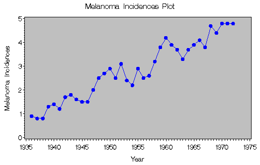
The time series data analyzed in this example are annual age-adjusted melanoma incidences from the Connecticut Tumor Registry (Houghton, Flannery, and Viola 1980) for the years 1936 to 1972. The observations represent the number of melanoma cases per 100,000 people.
The following DATA step reads the data in and creates a date variable to label the measurements.
      data melanoma ;
         input Incidences @@ ;
         year = intnx('year','1jan1936'd,_n_-1) ;
         format year year4. ;
         label Incidences = 'Age Adjusted Incidences of Melanoma per 100,000';
         datalines ;
            0.9 0.8 0.8 1.3 1.4 1.2 1.7 1.8 1.6 1.5
            1.5 2.0 2.5 2.7 2.9 2.5 3.1 2.4 2.2 2.9
            2.5 2.6 3.2 3.8 4.2 3.9 3.7 3.3 3.7 3.9
            4.1 3.8 4.7 4.4 4.8 4.8 4.8
            ;
      run ;
Figure 1 shows a plot of the data.
|
Figure 1: Melanoma Incidences Plot
To analyze this series, a UCM that contains a trend component, a cycle component, and an irregular component is appropriate. A time series yt that follows such a UCM can be formally described as
where ![]() is the trend component,
is the trend component,
![]() is the cycle component, and
is the cycle component, and ![]() is the error term. The error term
is also called the irregular component, which is assumed to be a Gaussian white noise with variance
is the error term. The error term
is also called the irregular component, which is assumed to be a Gaussian white noise with variance ![]() . The trend
. The trend ![]() is modeled as a stochastic component with slowly
varying level and slope. Its evolution is described as follows:
is modeled as a stochastic component with slowly
varying level and slope. Its evolution is described as follows:

The disturbances ![]() and
and ![]() are assumed to be independent. There
are some interesting special cases of this trend model, obtained by setting one or both of the disturbance variances,
are assumed to be independent. There
are some interesting special cases of this trend model, obtained by setting one or both of the disturbance variances, ![]() and
and ![]() , equal to zero. If
, equal to zero. If ![]() is set equal to zero, then you get a
linear trend model with fixed slope. If
is set equal to zero, then you get a
linear trend model with fixed slope. If ![]() is set to zero, then the resulting model usually has a smoother trend. If both the variances are
set to zero, then the resulting model is the deterministic linear time trend,
is set to zero, then the resulting model usually has a smoother trend. If both the variances are
set to zero, then the resulting model is the deterministic linear time trend, ![]() .
.
The cycle component ![]() is modeled
as follows:
is modeled
as follows:
Here ![]() is the damping factor, where
is the damping factor, where
![]() and the
disturbances
and the
disturbances ![]() and
and ![]() are independent
are independent ![]() variables. This results in a
damped stochastic cycle that has time-varying amplitude and phase, and a fixed period equal to
variables. This results in a
damped stochastic cycle that has time-varying amplitude and phase, and a fixed period equal to ![]() .
.
The parameters of this UCM are the different disturbance variances, ![]() ,
, ![]() ,
, ![]() , and
, and ![]() ; the damping factor
; the damping factor ![]() ; and the frequency
; and the frequency ![]() .
.
The following syntax fits the UCM to the melanoma incidences series:
   proc ucm data = melanoma;
      id year interval = year;
      model Incidences ;
      irregular ;
      level ;
      slope ;
      cycle ;
   run ;
Begin by specifying the input data set in the PROC statement. Second, use the ID statement in conjunction with the INTERVAL= statement to specify the time interval between observations. Note that the values of the ID variable are extrapolated for the forecast observations based on the values of the INTERVAL= option. Next, the MODEL statement is used to specify the dependent variable. If there are any predictors in the model, they are specified in the MODEL statement on the right-hand side of the equation. Finally, the IRREGULAR statement is used to specify the irregular component, the LEVEL and SLOPE statements are used to specify the trend component, and the CYCLE statement is used to specify the cycle component. Notice that different components in the model are specified by separate statements and that each component statement has a different set of options, which can be found in the SAS/ETS User's Guide. These options are useful for specifying additional details about that component. The following output from the UCM procedure in Figure 2 shows the parameter estimates for this model.
Figure 2: Parameter EstimatesThe table shows that the disturbance variances for the level and slope components are highly insignificant. This suggests that a deterministic trend model may be more appropriate. The estimated period of the cycle is about 9.7 years. Interestingly, this is similar to another well-known cycle, the sun-spot activity cycle, which is known to have a period of 9 to 11 years. This provides some support for the claim that the melonama incidences are related to sun exposure. The estimate of the damping factor is 0.96, which is close to 1. This suggests that the periodic pattern of melanoma incidences does not diminish quickly.
The procedure outputs a variety of other statistics useful in model diagnostics, such as series forecasts and component estimates, which point toward the use of a deterministic trend model. You can construct this model with a fixed linear trend by holding the values of the level and slope disturbance variances fixed at zero. These types of modifications in the model specification are very easy to do in the UCM procedure. The following syntax illustrates some of this functionality.
   ods html ;
   ods graphics on ;
   proc ucm data = melanoma;
      id year interval = year;
      model Incidences ;
      irregular ;
      level variance=0 noest ;
      slope variance=0 noest ;
      cycle plot=smooth ;
      estimate back=5 plot=(normal acf);
      forecast lead=10 back=5 plot=decomp;
   run ;
   ods graphics off ;
   ods html close ;
The ID, MODEL, and IRREGULAR statements appear as they did in the first model. In this model, however, you specify some specific options in the remaining component statements:
- In the LEVEL and SLOPE statements, the variances are set to zero to create a model with a fixed linear trend. A NOEST option is also included in these statements to fix the values of the model parameters.
- In the CYCLE statement, you can use the PLOT= option to plot the smoothed estimate of the cycle component.
- In the ESTIMATE statement, you are able to control the span of observations used in parameter estimation using the BACK= option. In this particular model, you set BACK=5 to specify a hold-out sample of five observations, which are omitted from the estimation. You can also plot the residual diagnostic plots using the PLOT= option.
- In the FORECAST statement, you use the LEAD= option to specify the number of periods to forecast beyond the historical period. In this case, you select to produce 10 multi-step forecasts. The BACK= option tells PROC UCM to begin the multi-step forecast five observations back from the end of the historical data. This corresponds with the beginning of the hold-out sample period specified by the BACK= option on the ESTIMATE statement. Thus a total of 10 multi-step forecasts are produced (five corresponding with the hold-out sample and five additional forecasts into the future). Finally, use the PLOT= option to generate the series decomposition plots.
- The ODS graphics on; statement invokes the ODS graphics system. The PLOT options on the CYCLE and FORECAST statements in the code cause ODS to produce high-resolution plots of the specified components. The ODS graphics off; statement turns off the graphics system. Note that the ODS Graphics System is experimental in SAS 9 and 9.1.
The parameter estimates for the deterministic trend model are shown in Figure 3:
|
The UCM Procedure
|
||||||||||||||||||||||||||||||||||||
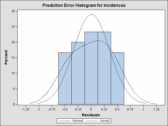
The procedure prints a variety of model diagnostic statistics by default (not shown). You can also request different residual plots. The model residual histogram and autocorrelation plots that follow in Figure 4 and Figure 5 do not show any serious violations of the model assumptions.
|
Figure 4: Prediction Error Histogram

|
Figure 5: Prediction Error Autocorrelations
The component plots in the model are useful for understanding the series' behavior and detecting structural breaks in the evolution of the series. The following plot in Figure 6 shows the smoothed estimate of the cycle component in the model.
|
Figure 6: Smoothed Cycle Component
You can also plot and print the series forecasts. The 10-year ahead forecasted values and their confidence intervals are shown in the following table in Figure 7. Remember that five measurements from the hold-out sample are included.
|
||||||||||||||||||||||||||||||||||||||||||||||||||||||||||||||||||||||||
The observations beyond the hold-out sample indicate that four to five incidences of melanoma per 100,000 people can be expected in the next five years.
You can also obtain a model-based "decomposition" of the series that shows the incremental effects of adding together different components that are present in the model. The following trend and trend plus cycle plots in Figure 8 and Figure 9 show such a decomposition in the current example.
|
Figure 8: Smoothed Trend Estimate
|
Figure 9: Sum of Trend and Cycle Components
The plot shows that the melanoma incidences are expected to increase over the next decade with some cyclical fluctuations.
References
Houghton, A. N., Flannery, J., and Viola, V. M. (1980), "Malignant Melanoma in Connecticut and Denmark," International Journal of Cancer, 25, 95-114.
SAS Institute Inc. (2002), SAS/ETS User's Guide, Version 9, Cary, NC: SAS Institute Inc.
These sample files and code examples are provided by SAS Institute Inc. "as is" without warranty of any kind, either express or implied, including but not limited to the implied warranties of merchantability and fitness for a particular purpose. Recipients acknowledge and agree that SAS Institute shall not be liable for any damages whatsoever arising out of their use of this material. In addition, SAS Institute will provide no support for the materials contained herein.
   /*-----------------------------------------------------------------
     Example: Analysis of Unobserved Component Models Using PROC UCM
     Requires: SAS/ETS
     Version: 9.0
     ------------------------------------------------------------------*/

   data melanoma ;
      input Incidences @@ ;
      year = intnx('year','1jan1936'd,_n_-1) ;
      format year year4. ;
      label Incidences = 'Age Adjusted Incidences of Melanoma per 100,000';
      datalines ;
         0.9 0.8 0.8 1.3 1.4 1.2 1.7 1.8 1.6 1.5
         1.5 2.0 2.5 2.7 2.9 2.5 3.1 2.4 2.2 2.9
         2.5 2.6 3.2 3.8 4.2 3.9 3.7 3.3 3.7 3.9
         4.1 3.8 4.7 4.4 4.8 4.8 4.8
         ;
   run ;


    proc gplot data = melanoma ;
       plot Incidences*year / cframe = ligr vaxis = axis1 haxis = axis2 ;
       title 'Melanoma Incidences Plot' ;
       symbol c = blue i = join v = dot ;
       axis1 label = (angle=90 'Melanoma Incidences') ;
       axis2 label =('Year') ;
    run ;


   proc ucm data = melanoma;
      id year interval = year;
      model Incidences ;
      irregular ;
      level ;
      slope ;
      cycle ;
   run ;


  ods html ;
  ods graphics on ;
   proc ucm data = melanoma;
      id year interval = year;
      model Incidences ;
      irregular ;
      level variance=0 noest ;
      slope variance=0 noest ;
      cycle plot=smooth ;
      estimate back=5 plot=(normal acf);
      forecast lead=10 back=5 plot=decomp;
   run ;
  ods graphics off ;
  ods html close ;
These sample files and code examples are provided by SAS Institute Inc. "as is" without warranty of any kind, either express or implied, including but not limited to the implied warranties of merchantability and fitness for a particular purpose. Recipients acknowledge and agree that SAS Institute shall not be liable for any damages whatsoever arising out of their use of this material. In addition, SAS Institute will provide no support for the materials contained herein.
| Type: | Sample |
| Topic: | SAS Reference ==> Procedures ==> UCM |
| Date Modified: | 2017-01-19 15:03:11 |
| Date Created: | 2017-01-19 14:57:10 |
Operating System and Release Information
| Product Family | Product | Host | SAS Release | |
| Starting | Ending | |||
| SAS System | SAS/ETS | z/OS | ||
| z/OS 64-bit | ||||
| OpenVMS VAX | ||||
| Microsoft® Windows® for 64-Bit Itanium-based Systems | ||||
| Microsoft Windows Server 2003 Datacenter 64-bit Edition | ||||
| Microsoft Windows Server 2003 Enterprise 64-bit Edition | ||||
| Microsoft Windows XP 64-bit Edition | ||||
| Microsoft® Windows® for x64 | ||||
| OS/2 | ||||
| Microsoft Windows 8 Enterprise 32-bit | ||||
| Microsoft Windows 8 Enterprise x64 | ||||
| Microsoft Windows 8 Pro 32-bit | ||||
| Microsoft Windows 8 Pro x64 | ||||
| Microsoft Windows 8.1 Enterprise 32-bit | ||||
| Microsoft Windows 8.1 Enterprise x64 | ||||
| Microsoft Windows 8.1 Pro 32-bit | ||||
| Microsoft Windows 8.1 Pro x64 | ||||
| Microsoft Windows 10 | ||||
| Microsoft Windows 95/98 | ||||
| Microsoft Windows 2000 Advanced Server | ||||
| Microsoft Windows 2000 Datacenter Server | ||||
| Microsoft Windows 2000 Server | ||||
| Microsoft Windows 2000 Professional | ||||
| Microsoft Windows NT Workstation | ||||
| Microsoft Windows Server 2003 Datacenter Edition | ||||
| Microsoft Windows Server 2003 Enterprise Edition | ||||
| Microsoft Windows Server 2003 Standard Edition | ||||
| Microsoft Windows Server 2003 for x64 | ||||
| Microsoft Windows Server 2008 | ||||
| Microsoft Windows Server 2008 R2 | ||||
| Microsoft Windows Server 2008 for x64 | ||||
| Microsoft Windows Server 2012 Datacenter | ||||
| Microsoft Windows Server 2012 R2 Datacenter | ||||
| Microsoft Windows Server 2012 R2 Std | ||||
| Microsoft Windows Server 2012 Std | ||||
| Microsoft Windows XP Professional | ||||
| Windows 7 Enterprise 32 bit | ||||
| Windows 7 Enterprise x64 | ||||
| Windows 7 Home Premium 32 bit | ||||
| Windows 7 Home Premium x64 | ||||
| Windows 7 Professional 32 bit | ||||
| Windows 7 Professional x64 | ||||
| Windows 7 Ultimate 32 bit | ||||
| Windows 7 Ultimate x64 | ||||
| Windows Millennium Edition (Me) | ||||
| Windows Vista | ||||
| Windows Vista for x64 | ||||
| 64-bit Enabled AIX | ||||
| 64-bit Enabled HP-UX | ||||
| 64-bit Enabled Solaris | ||||
| ABI+ for Intel Architecture | ||||
| AIX | ||||
| HP-UX | ||||
| HP-UX IPF | ||||
| IRIX | ||||
| Linux | ||||
| Linux for x64 | ||||
| Linux on Itanium | ||||
| OpenVMS Alpha | ||||
| OpenVMS on HP Integrity | ||||
| Solaris | ||||
| Solaris for x64 | ||||
| Tru64 UNIX | ||||