59730 - Poststratification with PROC SURVEYMEANS

Sample 59730: Poststratification with PROC SURVEYMEANS

PDF of Example | SAS/STAT Focus Area Examples

Overview

This example uses PROC SURVEYMEANS to obtain poststratified totals, means, and ratios. The data are sampled from county-level data sets that are publicly available from the USDA Economic Research Service website, at http://www.ers.usda.gov/data-products/county-level-data-sets.aspx. The sample consists of the county-level information about population size, the number of individuals in the labor force, and the number of unemployed persons in the 48 contiguous states of the United States of America in 2011. The sampling frame is stratified by state, and a simple random sample of two counties per state is selected. The analysis consists of a comparison between the non-poststratified estimates and the poststratified estimates of the total and average labor force size, number of unemployed, population size, and two ratios: the unemployment rate and the labor force participation rate. Table 1 describes the contents of the sample data set Unemployment, and Table 2 describes the interpretation of the six levels of the National Center for Health Statistics (NCHS) urban-rural classification for each county.

Table 1: Example Data Set Unemployment

Variable	Description
FIPS	Federal information processing standards (FIPS) code for counties
ST_FIPS	FIPS code for states
State	Abbreviation of state name
County	County name
Code2006	National Center for Health Statistics (NCHS) 2006 urban-rural classification code
Population	Resident total population estimate as of July 1, 2011
LaborForce	Number of individuals in the civilian labor force in 2011
Unemployed	Number of unemployed individuals in 2011
SamplingWeight	Sampling weight generated by yhe SURVEYSELECT procedure

Table 2: 2006 NCHS Urban-Rural Classification Scheme

Code	Urbanization Level	Classification Rules
1	Large metro, central	Counties in micropolitan statistical area (MSA) with population of 1 million
		or more that have the following characteristics:
		1) contain the entire population of the largest principal city of the MSA, or
		2) are completely contained within the largest principal city of the MSA, or
		3) contain at least 250,000 residents of any principal city in the MSA
2	Large metro, fringe	Counties in MSA with 1 million or more population that do not qualify as large central
3	Medium metro	Counties in MSA with 250,000–999,999 population
4	Small metro	Counties in MSA with 50,000–249,999 population
5	Micropolitan	Counties in micropolitan statistical area
6	Noncore	Counties not in micropolitan statistical area

The following SAS statements create the SAS data set Unemployment:


data unemployment;
  input FIPS 1-5 ST_FIPS 7-8 State $ 10-11 County $ 13-34 Code2006 35
        Population 37-45 LaborForce 46-52 Unemployed 53-58
        SamplingWeight 59-64;
  datalines;
1005  1  AL Barbour County        5 27313    9761   1110  33.5
1019  1  AL Cherokee County       6 26094    11696  1020  33.5
4021  4  AZ Pinal County          2 383553   139864 14466 7.5
4027  4  AZ Yuma County           4 200374   89500  24270 7.5
5105  5  AR Perry County          3 10384    4788   414   37.5

   ... more lines ...

55119 55 WI Taylor County         6 20759    10406  915   36.0
56025 56 WY Natrona County        4 76356    42907  2537  11.5
56037 56 WY Sweetwater County     5 44078    25138  1271  11.5
;
run;

You begin the comparative analysis by using PROC SURVEYMEANS as in the following statements to estimate the means, totals, and ratios of interest. The MEAN and SUM keywords in the PROC SURVEYMEANS statement request estimates of the population means and totals, respectively. The VAR statement requests estimates of the variables LaborForce, Unemployed, and Population. So, for example, if you specify the keyword MEAN in the PROC SURVEYMEANS statement and the variable Unemployed in the VAR statement, you are requesting an estimate of how many unemployed persons, on average, reside in a county. The first RATIO statement requests an estimate of the population’s unemployment rate, which is the ratio of the number of unemployed to the size of the labor force. The second RATIO statement requests an estimate of the labor force participation rate, which is the ratio of the size of the labor force to the size of the population of the county. The STRATA and WEIGHT statements identify the sampling design: the STRATA statement specifies that the strata are identified by the variable ST_FIPS, and the WEIGHT statement specifies that the sampling weights are contained in the variable SamplingWeight.


proc surveymeans data=unemployment mean sum;
  strata st_fips;
  weight SamplingWeight;
  var LaborForce Unemployed Population;
  ratio 'Unemployment Rate' Unemployed / LaborForce;
  ratio 'Labor Force Participation Rate' LaborForce / Population;
run;

Output 1 displays the estimated means, totals, ratios, and their standard errors. For example, on average there are 110,064 individuals in a county and 53,472 individuals in the labor force, and 4,925 individuals are unemployed. On average, the unemployment rate is 9.2%, and the labor force participation rate is 48.58%.

Output 1: Stratified Design

The SURVEYMEANS Procedure

Data Summary
Number of Strata	48
Number of Observations	96
Sum of Weights	3108

Statistics
Variable	Mean	Std Error of Mean	Sum	Std Dev
LaborForce	53472	6488.570784	166190527	20166478
Unemployed	4924.943050	594.657745	15306723	1848196
Population	110064	13105	342078597	40729501

Ratio Analysis: Unemployment Rate
Numerator	Denominator	Ratio	Std Err
Unemployed	LaborForce	0.092103	0.003090

Ratio Analysis: Labor Force Participation Rate
Numerator	Denominator	Ratio	Std Err
LaborForce	Population	0.485826	0.004186

In addition to the sample, the NCHS urban-rural classification code (Ingram and Franco, 2012) for each county in the sample and the total number of counties in the population that have each of the six levels of the NCHS classification are known. If the totals, means, and ratios of the variables of interest are homogeneous for counties that have the same NCHS urban-rural classification, but there is significant heterogeneity between counties whose classifications differ, then poststratifying by the NCHS urban-rural classification can potentially yield more efficient estimates.

The following SAS statements create the poststratum totals data set Poststrata. This data set is to be used in the PSTOTAL= option of the SURVEYMEANS procedure’s POSTSTRATA statement. A poststratum total data set must contain all the poststratification variables that are listed in the POSTSTRATA statement, and it must have a variable named _PSTOTAL_ that contains the poststratum totals. In the Poststrata data set, the variable Code2006 contains the poststratum identification code, and the variable _PSTOTAL_ contains the total number of counties in that poststratum in 2011.


data poststrata;
  input Code2006 _PSTOTAL_ ;
  datalines;
1 62
2 354
3 329
4 340
5 688
6 1336
;
run;

Figure 1 compares the distributions of Code2006 in the population and the weighted sample. Based on the weighted sample, counties that have values of 3 and 4 are overrepresented in the sample, and counties that have values of 5 and 6 are underrepresented in the sample. Poststratifying on Code2006 reweights the data such that the poststratified weighted sample distribution of Code2006 equals the population distribution.

Figure 1: Population Distribution versus Weighted Sample Distribution of Code2006

Population Distribution versus Weighted Sample Distribution of Code2006

To perform a poststratified analysis, you simply add a POSTSTRATA statement to the SURVEYMEANS procedure, as in the following statements. Specifically, you designate Code2006 as the poststratification variable, and you specify the SAS data set Poststrata in the PSTOTAL= option. The OUT= option saves the poststratification weights to the SAS data set Pswgt.


proc surveymeans data=unemployment mean sum;
  strata st_fips;
  weight SamplingWeight;
  var LaborForce Unemployed Population;
  ratio 'Unemployment Rate' Unemployed / LaborForce;
  ratio 'Labor Force Participation Rate' LaborForce / Population;
  poststrata code2006 / pstotal=poststrata out=pswgt;
run;

Figure 2 shows the ratios of the poststratification weights to the original sampling weights for each category of Code2006. Poststratification reduces the weights for counties that have Code2006 values of 3 and 4 and increases the weights for counties that have Code2006 values of 5 and 6.

Figure 2: Ratio of Poststratification Weights to Sampling Weights

Ratio of Poststratification Weights to Sampling Weights

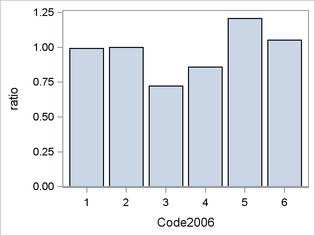
Figure 3 shows that, as expected, the poststratified weighted sample has the same distribution as the population.

Figure 3: Population Distribution versus Poststratified Weighted Sample Distribution of Code2006

Population Distribution versus Poststratified Weighted Sample Distribution of Code2006

Output 2 displays the poststratified estimates and their standard errors. All the poststratified estimates of the population means and totals are smaller than the non-poststratified estimates, but the two poststratified ratio estimates are larger. For example, the poststratified estimates indicate that on average there are 100,215 individuals in a county and 48,755 individuals in the labor force, and 4,518 individuals are unemployed. On average, the unemployment rate is 9.3%, and the labor force participation rate is 48.65%. Without exception, the variances of the estimates are smaller for the poststratified analysis, indicating that the poststratified estimates are more efficient for this sample.

Output 2: Poststratified Analysis

The SURVEYMEANS Procedure

Data Summary
Number of Strata	48
Number of Poststrata	6
Number of Observations	96
Sum of Weights	3108

Statistics
Variable	Mean	Std Error of Mean	Sum	Std Dev
LaborForce	48755	4808.671480	151579056	14950160
Unemployed	4517.976061	477.440072	14046388	1484361
Population	100215	9964.992605	311568502	30981162

Ratio Analysis: Unemployment Rate
Numerator	Denominator	Ratio	Std Err
Unemployed	LaborForce	0.092667	0.002727

Ratio Analysis: Labor Force Participation Rate
Numerator	Denominator	Ratio	Std Err
LaborForce	Population	0.486503	0.003853

Example: Age-Adjusted Mortality Rates

Suppose you want to compare the mortality rates of Florida and California. If you have samples from the two populations, computing the crude mortality rate for each population is straightforward. However, because many health outcomes vary by age and the two populations have different age distributions, a direct comparison of the crude mortality rates might be inappropriate. To make a relative comparison, you can use age-adjusted mortality rates. A common method of computing age-adjusted rates is called direct standardization; it is mathematically equivalent to poststratification.

The following SAS statements create the data sets Florida and California, which contain samples from a one-stage clustered sampling design that has a sampling rate of 0.5; the clusters consist of counties from the respective states, and the observations are age-specific groups. Each observation records the variable FIPS, which identifies the clusters (counties); the categorical variable Age, which identifies the age group; the variable Population, which records the total number of individuals in an age-specific group in 1968; the variable Deaths, which records the total number of recorded deaths in an age-specific group in 1968; and the variable SamplingWeights, which is the inverse of the probability of selecting a county in the sample. The data are sampled from the Compressed Mortality File (CMF), which is publicly available from the Centers for Disease Control and Prevention website, at http://www.cdc.gov/nchs/data_access/cmf.htm#data_availability.


data Florida;
   input FIPS Age Population Deaths;
   SamplingWeight=1.9705882353;
   datalines;
12011 4 7730 177
12011 5 32956 44
12011 6 49587 22
12011 7 49407 23
12011 8 40175 46
12011 9 29425 52

   ... more lines ...

12133 11 1048 5
12133 12 1149 13
12133 13 1252 20
12133 14 896 33
12133 15 425 33
12133 16 92 27
;


data California;
   input FIPS Age Population Deaths;
   SamplingWeight=2;
   datalines;
6001 4 17412 348
6001 5 72709 58
6001 6 101367 41
6001 7 95572 33
6001 8 89730 87
6001 9 107173 124

   ... more lines ...

6115 11 5421 11
6115 12 3720 34
6115 13 2766 58
6115 14 1752 77
6115 15 796 74
6115 16 180 39
;

Table 3 describes the different levels of the categorical variable Age.

Table 3: Age Categories

Age Category	Description
4	Less than 1 year
5	1–4 years
6	5–9 years
7	10–14 years
8	15–19 years
9	20–24 years
10	25–34 years
11	35–44 years
12	45–54 years
13	55–64 years
14	65–74 years
15	75–84 years
16	85+ years

The following SAS statements use the SURVEYMEANS procedure to estimate the crude mortality rates for Florida and California. The RATE= option in the PROC SURVEYMEANS statement identifies the sampling rate. The SURVEYMEANS procedure uses the sampling rate to compute a finite population correction for the Taylor series variance estimates. The RATIO and SUM keywords in the PROC SURVEYMEANS statement request estimates of the population ratios and totals, respectively. The VAR statement requests estimates of the variables Deaths and Population. The CLUSTER statement specifies that the variable FIPS identify the primary sampling units. The WEIGHT statement specifies that the variable SamplingWeight contain the sampling weights. The RATIO statement identifies the ratio of interest to be the number of deaths divided by the population size.


proc surveymeans data=Florida ratio sum rate=.5;
  cluster fips;
  weight SamplingWeight;
  var deaths population;
  ratio 'Florida Crude Mortality Rate' deaths/population;
run;


proc surveymeans data=California ratio sum rate=.5;
  cluster fips;
  weight SamplingWeight;
  var deaths population;
  ratio 'California Crude Mortality Rate' deaths/population;
run;

Output 3 and Output 4 show the estimation results.

Output 3: Crude Mortality Rate for Florida

Data Summary
Number of Clusters	34
Number of Observations	442
Sum of Weights	871

Ratio Analysis: Florida Crude Mortality Rate
Numerator	Denominator	Ratio	Std Err
Deaths	Population	0.010774	0.000464

Output 4: Crude Mortality Rate for California

Data Summary
Number of Clusters	29
Number of Observations	377
Sum of Weights	754

Ratio Analysis: California Crude Mortality Rate
Numerator	Denominator	Ratio	Std Err
Deaths	Population	0.007702	0.000595

The estimated crude mortality rates for Florida and California are 1.08% and 0.77%, respectively. The ratio of the crude mortality rates is 1.40. However, before you conclude that the mortality rate is higher in Florida than in California, consider the following two exhibits. Figure 4 shows that the age-specific mortality rates are decidedly a function of age in both states.

Figure 4: Age-Specific Crude Rates versus Age in Florida and California

Age-Specific Crude Rates versus Age in Florida and California

Figure 5 shows that the populations in Florida and California exhibit different age distributions. The percentage of residents in the age groups 13, 14, and 15 is higher in Florida than in California, whereas the percentage of residents in the age groups 5, 6, 7, 8, 9, 10, and 11 is lower in Florida than in California. Together these facts indicate that the crude mortality rates are not an appropriate measure for comparing differences between these two populations (Curtin and Klein, 1995).

Figure 5: Estimated Age Distributions in Florida and California

Estimated Age Distributions in Florida and California

Note: The SAS statements that generate Figure 4 and Figure 5 are not shown here but are included in the downloadable SAS program that is available with this web example.

Because the crude rate is not appropriate, and because age-specific mortality rates provide too much detail and require a large number of comparisons, you can use a summary measure that controls for a population’s age distribution. A commonly used measure is the age-adjusted mortality rate, which you can compute by performing direct standardization (Curtin and Klein, 1995).

As mentioned earlier, direct standardization is mathematically equivalent to poststratification. The difference between poststratification for the purpose of performing direct standardization and other forms of poststratification is this: when you perform direct standardization, the poststratum totals or proportions represent a standard or reference population rather than the population from which your sample was drawn.

To compute comparable age-adjusted rates for Florida and California by using poststratification, you need a data set that contains the age distribution proportions from a standard or reference population. The following SAS statements create the data set USbyAge, which contains the age-specific proportions for the US population in 1968:


data USbyAge;
  input Age _PSPCT_;
  datalines;
 4 0.01755
 5 0.07291
 6 0.10231
 7 0.10202
 8 0.09116
 9 0.07545
10 0.11879
11 0.11822
12 0.11391
13 0.09065
14 0.06103
15 0.02980
16 0.00621
;

You can then use PROC SUVEYMEANS to compute age-adjusted mortality rates for Florida and California. The procedure specification in the following SAS statements is the same as when you compute the crude rates, except that you add a POSTSTRATA statement, which specifies poststratification on the variable Age, and the PSPCT= option, which specifies that the population proportions be contained in the data set USbyAge.


proc surveymeans data=Florida ratio rate=.5;
  cluster fips;
  weight SamplingWeight;
  var deaths population;
  poststrata age / pspct=USbyAge;
  ratio 'Florida Standardized Mortality Rate' deaths/population;
run;


proc surveymeans data=California ratio rate=.5;
  cluster fips;
  weight SamplingWeight;
  var deaths population;
  poststrata age / pspct=USbyAge;
  ratio 'California Standardized Mortality Rate' deaths/population;
run;

Output 5 and Output 6 show the estimation results. The age-adjusted mortality rates for Florida and California are 0.70% and 0.48%, respectively. The ratio of the age-adjusted mortality rates is 1.45. Therefore, on an age-adjusted basis, the mortality rate in Florida in 1968 is almost 1.5 times the mortality rate in California in the same year.

Output 5: Standardized Mortality Rate for Florida

Data Summary
Number of Clusters	34
Number of Poststrata	13
Number of Observations	442
Sum of Weights	871

Ratio Analysis: Florida Standardized Mortality Rate
Numerator	Denominator	Ratio	Std Err
Deaths	Population	0.006952	0.000248

Output 6: Standardized Mortality Rate for California

Data Summary
Number of Clusters	29
Number of Poststrata	13
Number of Observations	377
Sum of Weights	754

Ratio Analysis: California Standardized Mortality Rate
Numerator	Denominator	Ratio	Std Err
Deaths	Population	0.004791	0.000385

References

Curtin, L. R. and Klein, R. J. (1995), “Direct Standardization (Age-Adjusted Death Rates),” Healthy People 2000: Statistical Notes, DHHS Publication No. (PHS) 95-1237.
Ingram, D. D. and Franco, S. J. (2012), “NCHS Urban-Rural Classification Scheme for Counties,” Vital and Health Statistics, Series 2: Data Evaluation and Methods Research no. 154, DHHS publication no. (PHS) 2012-1354.
Lehtonen, R. and Pahkinen, E. (2004), Practical Methods for Design and Analysis of Complex Surveys, 2nd Edition, Chichester, UK: John Wiley & Sons.
Lohr, S. L. (2010), Sampling: Design and Analysis, 2nd Edition, Boston: Brooks/Cole.
Särndal, C. E., Swensson, B., and Wretman, J. (1992), Model Assisted Survey Sampling, New York: Springer-Verlag.

These sample files and code examples are provided by SAS Institute Inc. "as is" without warranty of any kind, either express or implied, including but not limited to the implied warranties of merchantability and fitness for a particular purpose. Recipients acknowledge and agree that SAS Institute shall not be liable for any damages whatsoever arising out of their use of this material. In addition, SAS Institute will provide no support for the materials contained herein.

data unemployment;
  input FIPS 1-5 ST_FIPS 7-8 State $ 10-11 County $ 13-34 Code2006 35 
        Population 37-45 LaborForce 46-52 Unemployed 53-58 
        SamplingWeight 59-64;
  datalines;
1005  1  AL Barbour County        5 27313    9761   1110  33.5 
1019  1  AL Cherokee County       6 26094    11696  1020  33.5 
4021  4  AZ Pinal County          2 383553   139864 14466 7.5 
4027  4  AZ Yuma County           4 200374   89500  24270 7.5 
5105  5  AR Perry County          3 10384    4788   414   37.5 
5063  5  AR Independence County   5 36890    17068  1509  37.5 
6067  6  CA Sacramento County     1 1436262  675639 81541 29.0 
6013  6  CA Contra Costa County   2 1066516  524056 54451 29.0 
8003  8  CO Alamosa County        6 16103    8802   710   32.0 
8115  8  CO Sedgwick County       6 2377     1638   86    32.0 
9013  9  CT Tolland County        2 152487   87640  6467  4.0 
9009  9  CT New Haven County      3 862812   457666 44593 4.0 
10003 10 DE New Castle County     2 542444   271024 19913 1.5 
10005 10 DE Sussex County         5 200374   92577  6757  1.5 
12057 12 FL Hillsborough County   1 1269354  611769 64306 33.5 
12071 12 FL Lee County            3 631602   282699 31401 33.5 
13139 13 GA Hall County           4 182965   89960  7330  79.5 
13275 13 GA Thomas County         5 44724    21956  1813  79.5 
16023 16 ID Butte County          6 2816     1500   107   22.0 
16087 16 ID Washington County     6 10156    4831   490   22.0 
17007 17 IL Boone County          3 54253    26123  3519  51.0 
17127 17 IL Massac County         5 15359    7586   679   51.0 
18105 18 IN Monroe County         4 140063   70592  5028  46.0 
18131 18 IN Pulaski County        6 13307    6858   511   46.0 
19115 19 IA Louisa County         5 11361    5878   370   49.5 
19027 19 IA Carroll County        6 20829    12372  494   49.5 
20049 20 KS Elk County            6 2817     1530   108   52.5 
20063 20 KS Gove County           6 2699     1653   52    52.5 
21221 21 KY Trigg County          4 14235    6504   656   60.0 
21181 21 KY Nicholas County       6 7084     3209   329   60.0 
22031 22 LA De Soto Parish        3 26786    11291  877   32.0 
22047 22 LA Iberville Parish      3 33292    12523  1356  32.0 
23003 23 ME Aroostook County      6 71388    34542  3276  8.0 
23017 23 ME Oxford County         6 57771    28680  2768  8.0 
24037 24 MD St. Mary's County     5 107681   55648  3328  12.0 
24047 24 MD Worcester County      5 51446    28375  3463  12.0 
25021 25 MA Norfolk County        2 677683   363147 22630 7.0 
25023 25 MA Plymouth County       2 498275   262513 20401 7.0 
26123 26 MI Newaygo County        3 48432    21292  2199  41.5 
26039 26 MI Crawford County       6 14012    5874   658   41.5 
27163 27 MN Washington County     2 241511   133172 8089  43.5 
27023 27 MN Chippewa County       6 12314    7422   447   43.5 
28133 28 MS Sunflower County      5 28539    10528  1711  41.0 
28079 28 MS Leake County          6 23310    8544   1005  41.0 
29007 29 MO Audrain County        5 25593    11959  953   57.5 
29061 29 MO Daviess County        6 8315     4001   356   57.5 
30031 30 MT Gallatin County       5 91354    49513  3035  28.0 
30099 30 MT Teton County          6 6082     2950   160   28.0 
31149 31 NE Rock County           6 1428     920    25    46.5 
31183 31 NE Wheeler County        6 819      443    16    46.5 
32023 32 NV Nye County            5 43347    18138  2991  8.5 
32015 32 NV Lander County         6 5844     4458   293   8.5 
33001 33 NH Belknap County        5 60189    31669  1762  5.0 
33005 33 NH Cheshire County       5 76855    40744  2142  5.0 
34019 34 NJ Hunterdon County      2 127760   71262  4899  10.5 
34037 34 NJ Sussex County         2 148517   83728  7652  10.5 
35061 35 NM Valencia County       3 76842    30866  2692  16.5 
35025 35 NM Lea County            5 65136    29039  1508  16.5 
36071 36 NY Orange County         3 374438   173955 13606 31.0 
36025 36 NY Delaware County       6 47601    21469  1856  31.0 
37009 37 NC Ashe County           6 27139    12339  1505  50.0 
37187 37 NC Washington County     6 12960    6496   875   50.0 
38089 38 ND Stark County          5 25147    17136  343   26.5 
38097 38 ND Traill County         6 8060     4076   166   26.5 
39173 39 OH Wood County           3 126909   65549  5408  44.0 
39131 39 OH Pike County           6 28617    10627  1628  44.0 
40153 40 OK Woodward County       5 20055    12198  489   38.5 
40029 40 OK Coal County           6 5958     2686   202   38.5 
41017 41 OR Deschutes County      4 160083   80216  9917  18.0 
41045 41 OR Malheur County        5 30757    13555  1369  18.0 
42071 42 PA Lancaster County      3 523862   266366 18227 33.5 
42133 42 PA York County           3 437040   224969 17462 33.5 
44003 44 RI Kent County           2 165416   94995  10180 2.5 
44009 44 RI Washington County     2 126290   72461  6876  2.5 
45087 45 SC Union County          5 28630    11587  1873  23.0 
45089 45 SC Williamsburg County   6 34128    16175  2145  23.0 
46089 46 SD McPherson County      6 2449     1135   53    33.0 
46113 46 SD Shannon County        6 13909    3880   523   33.0 
47043 47 TN Dickson County        2 50094    25096  2405  47.5 
47147 47 TN Robertson County      2 66784    34888  2896  47.5 
48423 48 TX Smith County          4 212855   104089 8126  127.0 
48279 48 TX Lamb County           6 14130    6891   499   127.0 
49011 49 UT Davis County          3 311877   143526 8943  14.5 
49049 49 UT Utah County           3 530104   218763 14237 14.5 
50009 50 VT Essex County          5 6324     3143   240   7.0 
50027 50 VT Windsor County        5 56639    32490  1717  7.0 
51036 51 VA Charles City County   2 7258     3944   325   67.0 
51735 51 VA Poquoson city         2 12049    6658   361   67.0 
53067 53 WA Thurston County       4 256406   129026 10661 19.5 
53055 53 WA San Juan County       6 15812    7980   564   19.5 
54065 54 WV Morgan County         4 17454    7167   594   27.5 
54067 54 WV Nicholas County       6 26153    10714  968   27.5 
55049 55 WI Iowa County           3 23797    14126  908   36.0 
55119 55 WI Taylor County         6 20759    10406  915   36.0 
56025 56 WY Natrona County        4 76356    42907  2537  11.5 
56037 56 WY Sweetwater County     5 44078    25138  1271  11.5 
;
run;

proc surveymeans data=unemployment mean sum;
  strata st_fips;
  weight SamplingWeight;
  var LaborForce Unemployed Population;
  ratio 'Unemployment Rate' Unemployed / LaborForce;
  ratio 'Labor Force Participation Rate' LaborForce / Population;
run;

data poststrata;
  input Code2006 _PSTOTAL_ ;
  datalines;
1 62 
2 354 
3 329 
4 340 
5 688 
6 1336 
;
run;

proc sort data=unemployment out=unemployment;
  by code2006;
run;

ods select none;
proc means  data=unemployment;
  weight samplingweight;
  var code2006;
  by code2006;
  output out=sample N=sample sumwgt=sumwgt;
run;

data compare;
  merge poststrata sample(keep=code2006 sample sumwgt);
  by code2006;
run;

ods select none;
proc means data=compare;
 var _PSTOTAL_ ;
 output out=pop sum=sum ;
run;

data _null_;
  set pop;
  call symput('pop',sum);
run;

ods select none;
proc means data=compare;
  var sample ;
  output out=sample sum=sum ;
run;

data _null_;
  set sample;
  call symput('sample',sum);
run;

ods select none;
proc means data=compare;
  var sumwgt;
  output out=wgtsample sum=sum ;
run;

data _null_;
  set wgtsample;
  call symput('sumwgt',sum);
run;
   
data compare;
  set compare;
  _PSPCT_=_PSTOTAL_/&pop;
  samplepct=sample/&sample;
  wgtpct=sumwgt/&sumwgt;
run;

ods select all;

proc sgplot data=compare;
  vbar  code2006 / response=_PSPCT_ stat=sum 
                   legendlabel="Population" 
                   fillattrs=(color=red)
                   nostatlabel;
  vbar code2006 / response=samplepct stat=sum barwidth=.5 
                  legendlabel="Sample" 
                  fillattrs=(color=blue)
                  nostatlabel;
  yaxis label="Proportion";
run;

proc sgplot data=compare;
  vbar  code2006 / response=_PSPCT_ stat=sum 
                   legendlabel="Population" 
                   fillattrs=(color=red)
                   nostatlabel;
  vbar code2006 / response=wgtpct stat=sum barwidth=.5 
                  legendlabel="Sample" 
                  fillattrs=(color=blue)
                  nostatlabel;
  yaxis label="Proportion";
run;

proc surveymeans data=unemployment mean sum;
  strata st_fips;
  weight SamplingWeight;
  var LaborForce Unemployed Population;
  ratio 'Unemployment Rate' Unemployed / LaborForce;
  ratio 'Labor Force Participation Rate' LaborForce / Population;
  poststrata code2006 / pstotal=poststrata out=pswgt;
run;

data junk(keep=code2006 ratio);
  set pswgt(keep=code2006 samplingweight _pswt_);
  ratio=_pswt_/samplingweight;
run;

proc sgplot data=junk;
  vbar code2006 / response=ratio stat=mean nostatlabel;
run;

ods select none;
proc means  data=pswgt;
  weight _PSWt_;
  var code2006;
  by code2006;
  output out=pssample sumwgt=sumpswgt;
run;

data compare;
  merge compare pssample(keep=code2006 sumpswgt);
  by code2006;
run;

ods select none;
proc means data=compare;
  var sumpswgt ;
  output out=ps sum=sum ;
run;

data _null_;
  set ps;
  call symput('ps',sum);
run;

data compare;
  set compare;
  pspct=sumpswgt/&ps;
run;

ods select all;
proc sgplot data=compare;
  vbar  code2006 / response=_PSPCT_ stat=sum 
                   legendlabel="Population" 
                   fillattrs=(color=red)
                   nostatlabel;
  vbar code2006 / response=pspct stat=sum barwidth=.5 
                  legendlabel="Sample" 
                  fillattrs=(color=blue)
                  nostatlabel;
  yaxis label="Proportion";
run;

data Florida;
   input FIPS Age Population Deaths;
   SamplingWeight=1.9705882353;
   datalines;
12011 4 7730 177 
12011 5 32956 44 
12011 6 49587 22 
12011 7 49407 23 
12011 8 40175 46 
12011 9 29425 52 
12011 10 57198 120 
12011 11 64155 205 
12011 12 66692 475 
12011 13 71181 968 
12011 14 69139 1954 
12011 15 21787 1487 
12011 16 3030 494 
12013 4 140 4 
12013 5 592 0 
12013 6 792 1 
12013 7 881 2 
12013 8 726 3 
12013 9 391 2 
12013 10 780 2 
12013 11 720 3 
12013 12 904 8 
12013 13 851 20 
12013 14 479 18 
12013 15 225 22 
12013 16 45 11 
12015 4 156 6 
12015 5 821 1 
12015 6 1396 1 
12015 7 1498 0 
12015 8 1131 1 
12015 9 664 1 
12015 10 1410 2 
12015 11 1713 6 
12015 12 2342 27 
12015 13 4971 57 
12015 14 6498 200 
12015 15 1837 113 
12015 16 201 39 
12019 4 594 15 
12019 5 2456 4 
12019 6 3804 2 
12019 7 3321 2 
12019 8 2475 7 
12019 9 1943 4 
12019 10 4070 2 
12019 11 3398 9 
12019 12 2760 13 
12019 13 1789 27 
12019 14 1313 36 
12019 15 862 40 
12019 16 215 19 
12023 4 486 10 
12023 5 1818 2 
12023 6 2721 2 
12023 7 2795 1 
12023 8 2256 7 
12023 9 1583 6 
12023 10 2799 7 
12023 11 2671 17 
12023 12 2672 30 
12023 13 2056 33 
12023 14 1404 50 
12023 15 561 51 
12023 16 141 18 
12031 4 9870 219 
12031 5 38108 43 
12031 6 54855 23 
12031 7 55811 29 
12031 8 49014 54 
12031 9 49457 74 
12031 10 63968 120 
12031 11 63705 293 
12031 12 58752 555 
12031 13 41188 893 
12031 14 24777 1096 
12031 15 9977 827 
12031 16 2201 390 
12035 4 90 4 
12035 5 334 1 
12035 6 484 0 
12035 7 550 0 
12035 8 359 0 
12035 9 220 0 
12035 10 440 1 
12035 11 528 1 
12035 12 495 6 
12035 13 448 10 
12035 14 381 18 
12035 15 159 19 
12035 16 29 7 
12039 4 796 29 
12039 5 3043 5 
12039 6 4359 3 
12039 7 4469 3 
12039 8 3545 3 
12039 9 2027 3 
12039 10 3849 14 
12039 11 4090 27 
12039 12 4182 37 
12039 13 4150 71 
12039 14 2924 73 
12039 15 1382 66 
12039 16 389 29 
12041 4 50 0 
12041 5 231 0 
12041 6 371 0 
12041 7 351 0 
12041 8 247 0 
12041 9 175 0 
12041 10 399 1 
12041 11 334 1 
12041 12 395 2 
12041 13 343 7 
12041 14 202 9 
12041 15 122 6 
12041 16 31 4 
12043 4 52 5 
12043 5 284 0 
12043 6 420 0 
12043 7 414 0 
12043 8 275 1 
12043 9 182 1 
12043 10 422 1 
12043 11 358 1 
12043 12 403 4 
12043 13 297 10 
12043 14 184 11 
12043 15 54 4 
12043 16 15 1 
12049 4 304 7 
12049 5 1183 4 
12049 6 1518 2 
12049 7 1460 0 
12049 8 1312 2 
12049 9 858 2 
12049 10 1532 4 
12049 11 1565 5 
12049 12 1505 19 
12049 13 1258 21 
12049 14 823 36 
12049 15 450 42 
12049 16 91 26 
12063 4 490 11 
12063 5 2097 3 
12063 6 3155 3 
12063 7 3841 2 
12063 8 4106 6 
12063 9 2123 4 
12063 10 3536 8 
12063 11 3599 12 
12063 12 3593 51 
12063 13 3571 67 
12063 14 2267 96 
12063 15 1082 114 
12063 16 216 49 
12073 4 1676 35 
12073 5 6677 12 
12073 6 8944 12 
12073 7 8939 16 
12073 8 11355 13 
12073 9 14803 11 
12073 10 12765 19 
12073 11 9570 37 
12073 12 8652 66 
12073 13 5998 130 
12073 14 3229 146 
12073 15 1339 115 
12073 16 368 46 
12077 4 66 1 
12077 5 216 0 
12077 6 278 0 
12077 7 383 0 
12077 8 291 1 
12077 9 159 1 
12077 10 339 0 
12077 11 358 1 
12077 12 284 4 
12077 13 319 7 
12077 14 235 11 
12077 15 95 8 
12077 16 25 0 
12079 4 252 9 
12079 5 914 2 
12079 6 1250 2 
12079 7 1459 0 
12079 8 1622 1 
12079 9 772 1 
12079 10 1234 4 
12079 11 1219 3 
12079 12 1325 10 
12079 13 1413 27 
12079 14 942 20 
12079 15 431 44 
12079 16 119 14 
12081 4 1072 25 
12081 5 4352 6 
12081 6 6309 7 
12081 7 6937 2 
12081 8 6034 9 
12081 9 3796 7 
12081 10 6795 15 
12081 11 7961 37 
12081 12 8777 56 
12081 13 13169 187 
12081 14 17979 406 
12081 15 8299 460 
12081 16 1292 189 
12083 4 1164 32 
12083 5 4279 7 
12083 6 6191 3 
12083 7 6410 6 
12083 8 5340 7 
12083 9 3252 7 
12083 10 6415 16 
12083 11 6677 23 
12083 12 6676 63 
12083 13 6224 122 
12083 14 5190 220 
12083 15 2178 155 
12083 16 437 82 
12087 4 1160 28 
12087 5 3634 2 
12087 6 4717 1 
12087 7 4187 1 
12087 8 3894 3 
12087 9 7641 7 
12087 10 6799 8 
12087 11 5637 23 
12087 12 5072 52 
12087 13 4400 80 
12087 14 2665 107 
12087 15 888 86 
12087 16 116 25 
12089 4 342 10 
12089 5 1558 1 
12089 6 2331 0 
12089 7 2464 1 
12089 8 1879 6 
12089 9 1065 2 
12089 10 2414 5 
12089 11 2339 8 
12089 12 2045 17 
12089 13 1624 41 
12089 14 910 40 
12089 15 374 31 
12089 16 81 17 
12091 4 1754 36 
12091 5 6764 3 
12091 6 10827 5 
12091 7 10776 6 
12091 8 7025 9 
12091 9 10138 15 
12091 10 13116 21 
12091 11 11629 25 
12091 12 7403 49 
12091 13 3512 50 
12091 14 1690 68 
12091 15 703 67 
12091 16 128 28 
12095 4 5702 153 
12095 5 21523 29 
12095 6 34364 17 
12095 7 34481 14 
12095 8 30146 36 
12095 9 21757 30 
12095 10 36004 49 
12095 11 41159 135 
12095 12 37634 268 
12095 13 25245 447 
12095 14 19708 613 
12095 15 10111 721 
12095 16 2009 359 
12097 4 340 8 
12097 5 1228 3 
12097 6 1875 2 
12097 7 1939 0 
12097 8 1476 3 
12097 9 1007 4 
12097 10 1979 4 
12097 11 2031 11 
12097 12 2277 18 
12097 13 2358 40 
12097 14 2887 80 
12097 15 1780 121 
12097 16 344 60 
12099 4 4918 137 
12099 5 21082 29 
12099 6 29833 13 
12099 7 29961 16 
12099 8 24933 28 
12099 9 18826 28 
12099 10 33952 70 
12099 11 36034 135 
12099 12 36840 305 
12099 13 37215 622 
12099 14 32579 1019 
12099 15 13993 913 
12099 16 2333 356 
12101 4 664 19 
12101 5 2534 6 
12101 6 3936 3 
12101 7 3871 4 
12101 8 3577 7 
12101 9 2683 5 
12101 10 4019 5 
12101 11 4364 25 
12101 12 5391 59 
12101 13 9886 163 
12101 14 15296 378 
12101 15 5019 316 
12101 16 675 101 
12107 4 626 23 
12107 5 2523 2 
12107 6 3843 2 
12107 7 4013 1 
12107 8 3104 5 
12107 9 1862 8 
12107 10 3348 9 
12107 11 3851 17 
12107 12 3598 37 
12107 13 3123 67 
12107 14 2609 110 
12107 15 1080 67 
12107 16 222 45 
12113 4 780 16 
12113 5 2601 3 
12113 6 3860 1 
12113 7 3931 4 
12113 8 3098 6 
12113 9 4729 7 
12113 10 4783 5 
12113 11 3935 11 
12113 12 3157 32 
12113 13 2204 37 
12113 14 1372 49 
12113 15 600 50 
12113 16 99 26 
12115 4 1072 18 
12115 5 4415 4 
12115 6 7008 4 
12115 7 7627 6 
12115 8 6937 10 
12115 9 4102 7 
12115 10 7834 8 
12115 11 9813 36 
12115 12 11364 89 
12115 13 16604 244 
12115 14 21203 570 
12115 15 7936 504 
12115 16 1155 213 
12117 4 1324 30 
12117 5 5874 10 
12117 6 8687 4 
12117 7 8552 7 
12117 8 6487 8 
12117 9 3886 4 
12117 10 8634 10 
12117 11 9216 26 
12117 12 8607 70 
12117 13 6001 99 
12117 14 4506 149 
12117 15 2151 139 
12117 16 332 55 
12119 4 236 8 
12119 5 916 1 
12119 6 1337 0 
12119 7 1369 1 
12119 8 1396 2 
12119 9 886 3 
12119 10 1442 0 
12119 11 1278 8 
12119 12 1606 22 
12119 13 1523 26 
12119 14 1119 48 
12119 15 467 41 
12119 16 111 14 
12121 4 280 7 
12121 5 1046 1 
12121 6 1518 0 
12121 7 1577 0 
12121 8 1420 2 
12121 9 803 3 
12121 10 1461 5 
12121 11 1478 10 
12121 12 1669 15 
12121 13 1586 36 
12121 14 1029 40 
12121 15 566 42 
12121 16 133 24 
12123 4 278 5 
12123 5 1014 0 
12123 6 1520 0 
12123 7 1685 1 
12123 8 1339 2 
12123 9 813 2 
12123 10 1462 2 
12123 11 1683 6 
12123 12 1489 15 
12123 13 1368 23 
12123 14 805 30 
12123 15 328 21 
12123 16 77 12 
12127 4 2190 76 
12127 5 8438 6 
12127 6 12870 4 
12127 7 13833 1 
12127 8 12671 15 
12127 9 8844 16 
12127 10 13283 23 
12127 11 16026 60 
12127 12 17567 145 
12127 13 19228 382 
12127 14 21797 763 
12127 15 11464 790 
12127 16 1936 377 
12131 4 244 8 
12131 5 907 2 
12131 6 1329 2 
12131 7 1720 3 
12131 8 1381 3 
12131 9 844 1 
12131 10 1418 4 
12131 11 1670 11 
12131 12 1692 19 
12131 13 1801 26 
12131 14 1234 49 
12131 15 588 52 
12131 16 111 24 
12133 4 172 8 
12133 5 752 2 
12133 6 1135 1 
12133 7 1146 0 
12133 8 960 0 
12133 9 562 1 
12133 10 1127 3 
12133 11 1048 5 
12133 12 1149 13 
12133 13 1252 20 
12133 14 896 33 
12133 15 425 33 
12133 16 92 27 
;

data California;
   input FIPS Age Population Deaths;
   SamplingWeight=2;
   datalines;
6001 4 17412 348 
6001 5 72709 58 
6001 6 101367 41 
6001 7 95572 33 
6001 8 89730 87 
6001 9 107173 124 
6001 10 142762 225 
6001 11 121412 416 
6001 12 123592 945 
6001 13 89542 1439 
6001 14 57847 2077 
6001 15 31844 2411 
6001 16 7669 1342 
6005 4 140 3 
6005 5 565 0 
6005 6 904 3 
6005 7 928 0 
6005 8 1526 0 
6005 9 615 0 
6005 10 1081 2 
6005 11 1039 3 
6005 12 1395 12 
6005 13 1356 28 
6005 14 907 36 
6005 15 399 39 
6005 16 115 17 
6007 4 1332 24 
6007 5 5442 13 
6007 6 9043 2 
6007 7 9035 5 
6007 8 9129 10 
6007 9 8935 10 
6007 10 9566 14 
6007 11 9800 25 
6007 12 11226 68 
6007 13 10184 165 
6007 14 8168 297 
6007 15 4477 341 
6007 16 925 180 
6015 4 244 6 
6015 5 951 3 
6015 6 1558 3 
6015 7 1736 0 
6015 8 1232 6 
6015 9 763 2 
6015 10 1547 4 
6015 11 1713 4 
6015 12 1742 8 
6015 13 1375 15 
6015 14 908 27 
6015 15 299 21 
6015 16 70 13 
6017 4 514 5 
6017 5 2353 3 
6017 6 4177 2 
6017 7 4530 0 
6017 8 3571 4 
6017 9 2310 7 
6017 10 4518 9 
6017 11 5365 13 
6017 12 5463 33 
6017 13 4401 59 
6017 14 2741 77 
6017 15 972 82 
6017 16 167 37 
6023 4 1498 28 
6023 5 6359 4 
6023 6 10312 6 
6023 7 10690 5 
6023 8 10199 14 
6023 9 8497 6 
6023 10 11661 22 
6023 11 11417 43 
6023 12 11666 77 
6023 13 8919 145 
6023 14 5204 168 
6023 15 2562 214 
6023 16 583 105 
6025 4 1664 40 
6025 5 6272 4 
6025 6 9508 4 
6025 7 9381 4 
6025 8 7451 13 
6025 9 4185 12 
6025 10 8162 24 
6025 11 9022 44 
6025 12 7515 72 
6025 13 6258 110 
6025 14 3400 121 
6025 15 1327 121 
6025 16 288 53 
6029 4 5792 125 
6029 5 23655 20 
6029 6 37165 10 
6029 7 36749 16 
6029 8 31075 57 
6029 9 21118 44 
6029 10 39518 74 
6029 11 39298 123 
6029 12 36412 281 
6029 13 28117 467 
6029 14 16176 623 
6029 15 6883 605 
6029 16 1307 241 
6031 4 1320 23 
6031 5 5549 6 
6031 6 8231 1 
6031 7 7246 1 
6031 8 6112 8 
6031 9 7435 10 
6031 10 9162 11 
6031 11 7124 16 
6031 12 6063 43 
6031 13 4734 78 
6031 14 2633 89 
6031 15 1442 114 
6031 16 334 44 
6041 4 3104 53 
6041 5 14444 8 
6041 6 21776 5 
6041 7 20574 4 
6041 8 16784 17 
6041 9 14829 21 
6041 10 31739 33 
6041 11 29910 70 
6041 12 26777 149 
6041 13 16844 229 
6041 14 8970 273 
6041 15 4423 306 
6041 16 1072 185 
6043 4 58 1 
6043 5 257 0 
6043 6 488 1 
6043 7 423 0 
6043 8 444 1 
6043 9 271 2 
6043 10 503 0 
6043 11 529 2 
6043 12 647 5 
6043 13 709 13 
6043 14 644 23 
6043 15 221 19 
6043 16 68 12 
6047 4 2098 48 
6047 5 7698 9 
6047 6 11963 10 
6047 7 12062 4 
6047 8 9747 12 
6047 9 8092 12 
6047 10 11555 26 
6047 11 12220 37 
6047 12 10499 66 
6047 13 7619 133 
6047 14 4586 166 
6047 15 2125 177 
6047 16 428 77 
6049 4 92 0 
6049 5 384 0 
6049 6 685 0 
6049 7 745 1 
6049 8 660 2 
6049 9 340 1 
6049 10 741 3 
6049 11 824 4 
6049 12 969 4 
6049 13 839 10 
6049 14 550 14 
6049 15 254 18 
6049 16 40 13 
6051 4 52 0 
6051 5 206 0 
6051 6 335 0 
6051 7 320 1 
6051 8 306 0 
6051 9 203 0 
6051 10 406 2 
6051 11 519 1 
6051 12 448 6 
6051 13 425 8 
6051 14 203 4 
6051 15 39 2 
6051 16 9 2 
6053 4 4544 91 
6053 5 16664 10 
6053 6 22573 13 
6053 7 22473 9 
6053 8 29184 23 
6053 9 34987 29 
6053 10 28597 46 
6053 11 26093 72 
6053 12 23205 170 
6053 13 17410 259 
6053 14 10886 323 
6053 15 5123 371 
6053 16 1101 172 
6055 4 1086 18 
6055 5 4587 8 
6055 6 6964 4 
6055 7 7254 6 
6055 8 6576 12 
6055 9 5204 7 
6055 10 8049 8 
6055 11 8470 20 
6055 12 9686 45 
6055 13 7894 118 
6055 14 5938 183 
6055 15 3441 214 
6055 16 707 132 
6059 4 24168 433 
6059 5 105786 70 
6059 6 158352 54 
6059 7 152819 44 
6059 8 120630 110 
6059 9 97679 93 
6059 10 185414 185 
6059 11 187199 390 
6059 12 148622 773 
6059 13 78301 1052 
6059 14 54667 1601 
6059 15 27755 1952 
6059 16 5537 893 
6061 4 1046 33 
6061 5 4450 4 
6061 6 7278 4 
6061 7 7973 1 
6061 8 7215 11 
6061 9 4010 11 
6061 10 7999 20 
6061 11 9390 16 
6061 12 9321 60 
6061 13 7269 91 
6061 14 4787 134 
6061 15 2288 182 
6061 16 430 79 
6063 4 170 5 
6063 5 603 1 
6063 6 1082 0 
6063 7 1170 0 
6063 8 980 2 
6063 9 462 2 
6063 10 1024 5 
6063 11 1514 6 
6063 12 1605 10 
6063 13 1440 23 
6063 14 802 28 
6063 15 334 30 
6063 16 36 15 
6069 4 380 6 
6069 5 1446 2 
6069 6 1964 2 
6069 7 1838 0 
6069 8 1731 2 
6069 9 1104 1 
6069 10 1931 5 
6069 11 1989 6 
6069 12 1898 13 
6069 13 1624 34 
6069 14 1072 31 
6069 15 612 54 
6069 16 123 23 
6075 4 11120 203 
6075 5 39094 28 
6075 6 48010 24 
6075 7 46518 26 
6075 8 50731 56 
6075 9 74966 99 
6075 10 103744 188 
6075 11 83917 349 
6075 12 88893 872 
6075 13 88891 1735 
6075 14 63294 2234 
6075 15 29352 2377 
6075 16 6030 1205 
6083 4 4378 77 
6083 5 17753 11 
6083 6 26489 6 
6083 7 25618 7 
6083 8 25544 19 
6083 9 27319 21 
6083 10 32930 41 
6083 11 30549 77 
6083 12 25990 154 
6083 13 19050 270 
6083 14 13602 417 
6083 15 7079 498 
6083 16 1601 267 
6085 4 18746 289 
6085 5 84608 60 
6085 6 120233 28 
6085 7 109430 27 
6085 8 90363 75 
6085 9 83824 108 
6085 10 154686 122 
6085 11 131384 256 
6085 12 109145 623 
6085 13 62386 842 
6085 14 35542 1097 
6085 15 18947 1374 
6085 16 4422 723 
6093 4 514 8 
6093 5 2043 1 
6093 6 3084 1 
6093 7 3404 1 
6093 8 3104 3 
6093 9 1762 5 
6093 10 3401 5 
6093 11 4074 18 
6093 12 4380 29 
6093 13 3680 54 
6093 14 2406 86 
6093 15 1049 85 
6093 16 229 42 
6095 4 3346 85 
6095 5 12503 6 
6095 6 17551 5 
6095 7 16256 13 
6095 8 14729 15 
6095 9 20789 26 
6095 10 21492 29 
6095 11 19026 55 
6095 12 17190 113 
6095 13 11186 185 
6095 14 6924 277 
6095 15 3148 243 
6095 16 551 102 
6101 4 782 13 
6101 5 2951 1 
6101 6 4625 2 
6101 7 4472 1 
6101 8 3872 8 
6101 9 2615 7 
6101 10 5166 4 
6101 11 4938 13 
6101 12 4438 36 
6101 13 3630 68 
6101 14 1951 72 
6101 15 1047 95 
6101 16 247 43 
6105 4 114 2 
6105 5 430 2 
6105 6 736 1 
6105 7 862 0 
6105 8 577 0 
6105 9 293 1 
6105 10 790 1 
6105 11 803 3 
6105 12 1003 7 
6105 13 894 12 
6105 14 484 13 
6105 15 175 8 
6105 16 41 11 
6111 4 6662 138 
6111 5 30025 25 
6111 6 45978 10 
6111 7 41907 14 
6111 8 32286 35 
6111 9 22998 40 
6111 10 49258 58 
6111 11 47749 136 
6111 12 36109 221 
6111 13 21806 320 
6111 14 14113 452 
6111 15 6604 459 
6111 16 1394 224 
6115 4 1004 15 
6115 5 3628 3 
6115 6 5489 6 
6115 7 5014 1 
6115 8 3630 5 
6115 9 4539 9 
6115 10 6330 5 
6115 11 5421 11 
6115 12 3720 34 
6115 13 2766 58 
6115 14 1752 77 
6115 15 796 74 
6115 16 180 39 
;

ods output DomainRatio=fldomain(keep=age ratio rename=(ratio=florida))
           Domain=fl_agepop(where=(varname="Population") keep=age sum varname) 
           Statistics=fl_pop(where=(varname="Population") keep=sum varname);
proc surveymeans data=Florida ratio sum rate=.5;
  cluster fips;
  weight SamplingWeight;
  var deaths population;
  domain age;
  ratio 'Florida Crude Mortality Rate' deaths/population;
run;

ods output DomainRatio=cadomain(keep=age ratio rename=(ratio=california))
           Domain=ca_agepop(where=(varname="Population") keep=age sum varname) 
           Statistics=ca_pop(where=(varname="Population") keep=sum varname);
proc surveymeans data=California ratio sum rate=.5;
  cluster fips;
  weight SamplingWeight;
  var deaths population;
  domain age;
  ratio 'California Crude Mortality Rate' deaths/population;
run;

data fl_agepop;
  set fl_agepop(rename=(sum=fl_sum) drop=varname);
  index=1;
run;

data fl_pop;
  set fl_pop(rename=(sum=fl_pop) drop=varname);
  index=1;
run;

data fl_agepct(drop=index fl_pop);
  merge fl_agepop fl_pop;
  by index;
  fl_pct=fl_sum/fl_pop;
run;

data ca_agepop;
  set ca_agepop(rename=(sum=ca_sum) drop=varname);
  index=1;
run;

data ca_pop;
  set ca_pop(rename=(sum=ca_pop) drop=varname);
  index=1;
run;

data ca_agepct(drop=index ca_pop);
  merge ca_agepop ca_pop;
  by index;
  ca_pct=ca_sum/ca_pop;
run;

data age;
  merge ca_agepct fl_agepct;
  by age;
run;

proc sgplot data=age;
  vbar age / response=ca_pct stat=sum 
             legendlabel="California" 
             fillattrs=(color=red) nostatlabel;
  vbar age / response=fl_pct stat=sum barwidth=.5 
             legendlabel="Florida" 
             fillattrs=(color=blue) nostatlabel;
  yaxis label="Proportion";
             
run;

data domain;
  merge fldomain cadomain;
  by age;
run;

proc sgplot data=domain;
  series x=age y=Florida / legendlabel="Florida";
  series x=age y=California / legendlabel="California";
  xaxis integer;
  yaxis label="Crude Rate";
run;

data USbyAge;
  input Age _PSPCT_;
  datalines;
 4 0.01755 
 5 0.07291 
 6 0.10231 
 7 0.10202 
 8 0.09116 
 9 0.07545 
10 0.11879 
11 0.11822 
12 0.11391 
13 0.09065 
14 0.06103 
15 0.02980 
16 0.00621 
;

proc surveymeans data=Florida ratio rate=.5;
  cluster fips;
  weight SamplingWeight;
  var deaths population;
  poststrata age / pspct=USbyAge;
  ratio 'Florida Standardized Mortality Rate' deaths/population;
run;

proc surveymeans data=California ratio rate=.5;
  cluster fips;
  weight SamplingWeight;
  var deaths population;
  poststrata age / pspct=USbyAge;
  ratio 'California Standardized Mortality Rate' deaths/population;
run;

These sample files and code examples are provided by SAS Institute Inc. "as is" without warranty of any kind, either express or implied, including but not limited to the implied warranties of merchantability and fitness for a particular purpose. Recipients acknowledge and agree that SAS Institute shall not be liable for any damages whatsoever arising out of their use of this material. In addition, SAS Institute will provide no support for the materials contained herein.

This example uses PROC SURVEYMEANS to obtain poststratified totals, means, and ratios.

Type:	Sample
Topic:	SAS Reference ==> Procedures ==> SURVEYMEANS Analytics ==> Survey Sampling and Analysis

Date Modified:	2017-01-18 09:38:10
Date Created:	2017-01-18 09:31:57

Operating System and Release Information

Product Family	Product	Host	SAS Release
Product Family	Product	Host	Starting	Ending
SAS System	SAS/STAT	z/OS
		z/OS 64-bit
		OpenVMS VAX
		Microsoft® Windows® for 64-Bit Itanium-based Systems
		Microsoft Windows Server 2003 Datacenter 64-bit Edition
		Microsoft Windows Server 2003 Enterprise 64-bit Edition
		Microsoft Windows XP 64-bit Edition
		Microsoft® Windows® for x64
		OS/2
		Microsoft Windows 8 Enterprise 32-bit
		Microsoft Windows 8 Enterprise x64
		Microsoft Windows 8 Pro 32-bit
		Microsoft Windows 8 Pro x64
		Microsoft Windows 8.1 Enterprise 32-bit
		Microsoft Windows 8.1 Enterprise x64
		Microsoft Windows 8.1 Pro 32-bit
		Microsoft Windows 8.1 Pro x64
		Microsoft Windows 10
		Microsoft Windows 95/98
		Microsoft Windows 2000 Advanced Server
		Microsoft Windows 2000 Datacenter Server
		Microsoft Windows 2000 Server
		Microsoft Windows 2000 Professional
		Microsoft Windows NT Workstation
		Microsoft Windows Server 2003 Datacenter Edition
		Microsoft Windows Server 2003 Enterprise Edition
		Microsoft Windows Server 2003 Standard Edition
		Microsoft Windows Server 2003 for x64
		Microsoft Windows Server 2008
		Microsoft Windows Server 2008 R2
		Microsoft Windows Server 2008 for x64
		Microsoft Windows Server 2012 Datacenter
		Microsoft Windows Server 2012 R2 Datacenter
		Microsoft Windows Server 2012 R2 Std
		Microsoft Windows Server 2012 Std
		Microsoft Windows XP Professional
		Windows 7 Enterprise 32 bit
		Windows 7 Enterprise x64
		Windows 7 Home Premium 32 bit
		Windows 7 Home Premium x64
		Windows 7 Professional 32 bit
		Windows 7 Professional x64
		Windows 7 Ultimate 32 bit
		Windows 7 Ultimate x64
		Windows Millennium Edition (Me)
		Windows Vista
		Windows Vista for x64
		64-bit Enabled AIX
		64-bit Enabled HP-UX
		64-bit Enabled Solaris
		ABI+ for Intel Architecture
		AIX
		HP-UX
		HP-UX IPF
		IRIX
		Linux
		Linux for x64
		Linux on Itanium
		OpenVMS Alpha
		OpenVMS on HP Integrity
		Solaris
		Solaris for x64
		Tru64 UNIX

Support

Sample 59730: Poststratification with PROC SURVEYMEANS

Overview

Example: Age-Adjusted Mortality Rates

References

Operating System and Release Information