Usage Note 57480: Modeling continuous proportions: Normal and Beta Regression Models
 |  |  |
Researchers who conduct clinical trials often have to measure the concentration of a drug in a patient’s blood over a specified interval of time. The measured data represents the body’s reaction as evidenced by an increase or decrease in the concentration of a particular substance. Another example occurs when scientists gather data to measure the concentration of a toxin from a chemical spill that poses an acute risk of cancer and neurological effects as well as many other negative health impacts including heart damage, lung disease, kidney disease, reproductive problems, gastrointestinal illness, birth defects, or impaired bone growth in children. Such response measures are proportions that vary continuously over the zero to one range (or zero to 100 when percentages).
While the binomial distribution is generally applicable to a dependent (response) variable that represents proportions from aggregated binary responses, it might not apply to underlying continuous data. The binomial distribution is typically used when the proportions represent a count of events resulting from a known number of trials. Response measurements, like those above, that are proportions relative to a standard (such as proportion of control) or percentages of a total amount (such as proportion reduction in body fat, proportion of area damaged in a forest fire, proportion of chemical absorbed, or the amount of funds charged off out of a balance) might not be binomial since they do not represent a set of independent trials. When the response in a regression model is a proportion or a percentage, it can be difficult to decide on an appropriate modeling approach. While some researchers use the simplest approach and fit a linear regression model, ordinary linear regression can predict invalid values that are less than zero or greater than one. Proportion data typically exhibit a sigmoidal, or S-shaped, curve with asymptotes at the limits of zero and one when plotted against a predictor. In general, ordinary regression does not capture this relationship, but it might be reasonable if all of the data fall in the middle of the range (between about 0.3 and 0.7) where the curve is approximately linear. However, there are other approaches that can be used.
Two ways to model continuous proportions include using the beta distribution in the GLIMMIX procedure or defining a nonlinear model using the NLIN or NLMIXED procedures in SAS/STAT® software. The following examples illustrate these approaches using the GLIMMIX and NLIN procedures to model continuous proportions or percentages. Two other models are the fractional logistic model, which uses a quasi-likelihood approach, and the 4- or 5-parameter logistic model also known as Emax models. These models are discussed and illustrated in this note.
The following statements create the data set with tissue damage proportions, Y, at various concentrations of the chemical, CONC. Note that the concentrations are approximately equally spaced on the common log scale.
      data damage;
        input conc y;
        lconc=log10(conc);
        datalines;
      0.1   .08
      0.25  .09
      0.5   .11
      1.0   .20
      2     .30
      4     .53
      5.0   .63
      8.0   .71
      10.0  .73
      25.0  .84
      50.0  .85
      100.0 .86
      ;
Normal model: REG and NLIN procedures
These statements fit a simple linear regression model using the REG procedure. The OUTPUT statement saves the predicted responses in data set REGOUT.
      proc reg data=damage;
        model y = lconc;
        output out=regout p=rpredy;
        quit;
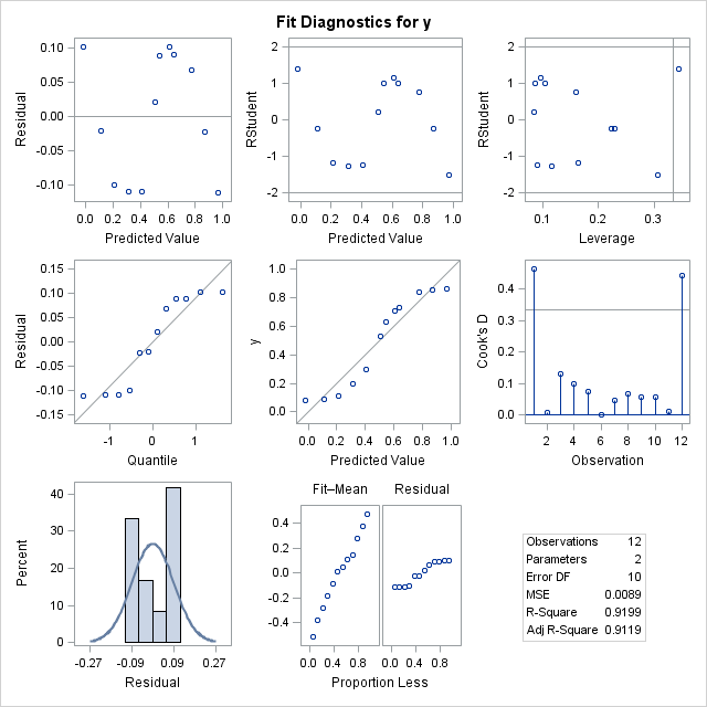
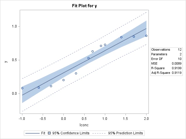
The model produces the following graphical results. Even though the fit plot does not look too bad and R2 is high (0.9119), the diagnostic plots indicate possible problems with the model fit. The residuals are not randomly scattered about zero, the residual quantile plot indicates possible violation of the normality assumption, and the plot of the response variable Y against the predicted values look more like an S-shaped curve than a straight line. Also, examination of the data set of predicted values shows that one of the values falls outside the [0,1] range.
|
Under the assumption that the observed proportions are from a normal distribution, the following statements estimate a nonlinear logistic curve using the NLIN procedure. The logistic function is 1/(1+e-x) and maps values of x to the interval [0,1] for any real value of x. Since it produces values between zero and one, it is a reasonable candidate for a model on proportions.
      proc nlin data=damage plots=all hougaard;
        parms p1=1 p2=0.5;
        xbeta=p1 + p2*lconc;
        model y=1/(1 + exp(-xbeta));
        output out=nlinout p=npredy lclm=lower uclm=upper;
        run;
Following are the estimated parameters of the two-parameter logistic model. The skewness measures of -0.2889 and 0.3498 indicate that the parameter estimators exhibit skewed behavior and that their standard errors and confidence intervals should be used cautiously for inferences.
| ||||||||||||||||||
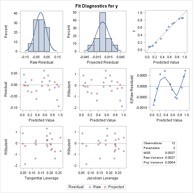
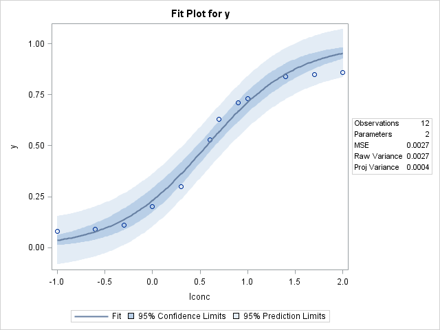
Notice that the fitted model does a better job of following the curvature of the observed proportions though the diagnostic plots still indicate problems similar to the linear regression model above.
|
Beta model: GLIMMIX procedure
Some researchers model continuous proportions using the beta distribution. Like proportions, the beta distribution supports a range from zero to one. The beta distribution can also accommodate right or left skewness, two conditions that the normal distribution cannot account for because of its symmetry. The GLIMMIX procedure fits a beta-logistic model using maximum likelihood estimation when the DIST=BETA and LINK=LOGIT options are specified in the MODEL statement. The logit link ensures that the predicted mean stays within bounds (0,1). However, this model does not permit proportions equal to 0 or 1. Such observations are ignored by GLIMMIX when fitting the beta model.
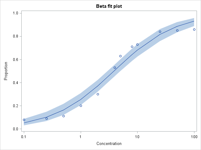
The following statements fit the beta-logistic model and save the predicted values and 95% confidence limits in data set GMXOUT.
      proc glimmix data=damage;
        model y = lconc / dist=beta link=logit solution;
        output out=gmxout pred(ilink)=gpredy lcl(ilink)=lower ucl(ilink)=upper;
        run;
The Dimensions table indicates one covariance parameter was estimated that corresponds to the scale parameter. The scale parameter (59.4261) is displayed in the Parameter Estimates table and is inversely related to the variance of the response variable. For models without random effects, a good model fit is indicated when the Pearson chi-square divided by its degrees of freedom is close to one. For this model the statistic is 1.38 suggesting that the model fits the data well. The regression parameters of the beta regression model are interpretable as log odds ratios when the logit link is used. The significant parameter estimate for lconc (p<0.0001) suggests that as the log concentration increases by one unit, the log odds of tissue damage increases by 1.8406. Equivalently, e1.8406=6.3 is the estimated odds ratio indicating that every one unit increase in the log concentration increases the odds of tissue damage by 6.3.
| ||||||||||||||||||||||||||||||||||||||||||||||||||||||||||||
These statements plot the fitted model.
      proc sgplot data=gmxout noautolegend;
        band upper=upper lower=lower x=conc;
        scatter y=y x=conc;
        series y=gpredy x=conc;
        xaxis type=log label="Concentration";
        yaxis label="Proportion";
        title "Beta fit plot";
        run;
As with the logistic model fit with NLIN, the beta model does a reasonable job of following the data curvature.
|
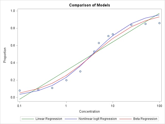
The following statements create a comparative plot of the models fit using the REG, NLIN and GLIMMIX procedures.
      data combo;
        merge regout nlinout gmxout;
        run;

      proc sgplot data=combo;
        scatter y=y x=conc;
        series y=rpredy x=conc / lineattrs=(color=green)
           name="Linear Regression" legendlabel="Linear Regression";
        series y=npredy x=conc / lineattrs=(color=blue)
           name="Nonlinear logit Regression" legendlabel="Nonlinear logit Regression";
        series y=gpredy x=conc / lineattrs=(color=red)
           name="Beta Regression" legendlabel="Beta Regression";
        xaxis type=log label="Concentration";
        yaxis label="Proportion";
        keylegend "Linear Regression" "Nonlinear logit Regression" "Beta Regression";
        title "Comparison of Models";
        run;
The normal-logistic model from NLIN and the beta-logistic model from GLIMMIX capture some of the curvature in the data. However, these data seem to plateau at both low and high proportions. Another model, the 4-parameter logistic model can model data that is limited to a portion of the [0,1] range, and is illustrated in this note.
|
The beta model can be used to fit more complex models to continuous proportion data. For example, the following statements fit a random effects model to simulated data collected on individuals in cities.
      proc glimmix method=quad plots=studentpanel;
        class city;
        model y = x / dist=beta link=logit solution;
        random intercept / subject=city solution;
        run;
Operating System and Release Information
| Product Family | Product | System | SAS Release | |
| Reported | Fixed* | |||
| SAS System | SAS/STAT | z/OS | ||
| z/OS 64-bit | ||||
| OpenVMS VAX | ||||
| Microsoft® Windows® for 64-Bit Itanium-based Systems | ||||
| Microsoft Windows Server 2003 Datacenter 64-bit Edition | ||||
| Microsoft Windows Server 2003 Enterprise 64-bit Edition | ||||
| Microsoft Windows XP 64-bit Edition | ||||
| Microsoft® Windows® for x64 | ||||
| OS/2 | ||||
| Microsoft Windows 8 Enterprise 32-bit | ||||
| Microsoft Windows 8 Enterprise x64 | ||||
| Microsoft Windows 8 Pro 32-bit | ||||
| Microsoft Windows 8 Pro x64 | ||||
| Microsoft Windows 8.1 Enterprise 32-bit | ||||
| Microsoft Windows 8.1 Enterprise x64 | ||||
| Microsoft Windows 8.1 Pro | ||||
| Microsoft Windows 8.1 Pro 32-bit | ||||
| Microsoft Windows 10 | ||||
| Microsoft Windows 95/98 | ||||
| Microsoft Windows 2000 Advanced Server | ||||
| Microsoft Windows 2000 Datacenter Server | ||||
| Microsoft Windows 2000 Server | ||||
| Microsoft Windows 2000 Professional | ||||
| Microsoft Windows NT Workstation | ||||
| Microsoft Windows Server 2003 Datacenter Edition | ||||
| Microsoft Windows Server 2003 Enterprise Edition | ||||
| Microsoft Windows Server 2003 Standard Edition | ||||
| Microsoft Windows Server 2003 for x64 | ||||
| Microsoft Windows Server 2008 | ||||
| Microsoft Windows Server 2008 R2 | ||||
| Microsoft Windows Server 2008 for x64 | ||||
| Microsoft Windows Server 2012 Datacenter | ||||
| Microsoft Windows Server 2012 R2 Datacenter | ||||
| Microsoft Windows Server 2012 R2 Std | ||||
| Microsoft Windows Server 2012 Std | ||||
| Microsoft Windows XP Professional | ||||
| Windows 7 Enterprise 32 bit | ||||
| Windows 7 Enterprise x64 | ||||
| Windows 7 Home Premium 32 bit | ||||
| Windows 7 Home Premium x64 | ||||
| Windows 7 Professional 32 bit | ||||
| Windows 7 Professional x64 | ||||
| Windows 7 Ultimate 32 bit | ||||
| Windows 7 Ultimate x64 | ||||
| Windows Millennium Edition (Me) | ||||
| Windows Vista | ||||
| Windows Vista for x64 | ||||
| 64-bit Enabled AIX | ||||
| 64-bit Enabled HP-UX | ||||
| 64-bit Enabled Solaris | ||||
| ABI+ for Intel Architecture | ||||
| AIX | ||||
| HP-UX | ||||
| HP-UX IPF | ||||
| IRIX | ||||
| Linux | ||||
| Linux for x64 | ||||
| Linux on Itanium | ||||
| OpenVMS Alpha | ||||
| OpenVMS on HP Integrity | ||||
| Solaris | ||||
| Solaris for x64 | ||||
| Tru64 UNIX | ||||
| Type: | Usage Note |
| Priority: | |
| Topic: | SAS Reference ==> Procedures ==> GLIMMIX SAS Reference ==> Procedures ==> NLIN SAS Reference ==> Procedures ==> REG Analytics ==> Regression |
| Date Modified: | 2016-02-03 16:40:44 |
| Date Created: | 2016-01-20 15:09:19 |