45566 - Bayesian Exponential Mixture Model

Sample 45566: Bayesian Exponential Mixture Model

PDF of Example | SAS/STAT Focus Area Examples

Analysis

The LOS data analyzed in this example originate from geriatric patients in a psychiatric hospital in North East London in 1991 and were studied by Harrison and Millard ( 1991 ) and McClean and Millard ( 1993 ) . Each observation represents the LOS in days for an admitted patient.

   data inputdata;
      input los @@;
      datalines;                                                                         
   1671 1300   722   586   552   525  364                                                
    359  321   302   272   248   226  216
    208  182   141   141   132   120  117
    115  114   113   104   103   101   99                                          
     96   94    93    92    88    84   83
     81   79    74    70    63    62   62
     61   56    55    53    53    51   51
     50   49    36    33    33    33   29
     28   26    24    19    16    16   15
   
   ... more lines ...   

     35   28    20    19     9     5    2
      2    2 22317 14006 11549 11006 8981
   8402 7947  7266  6693  4408  4010 4003
   1970 1857  1849  1833  1770  1769 1514
   1217  956   924   611   386   280   93
   ;

Before using this data in a mixture model setting, use the MEANS procedure to obtain summary statistics for the LOS data in table form. Figure 1 displays summary statistics for this data.

Figure 1 PROC MEANS Summary of LOS

The MEANS Procedure

Analysis Variable : los
N	Mean	Std Dev	Minimum	Maximum
469	3712.36	5675.97	1.0000000	24028.00

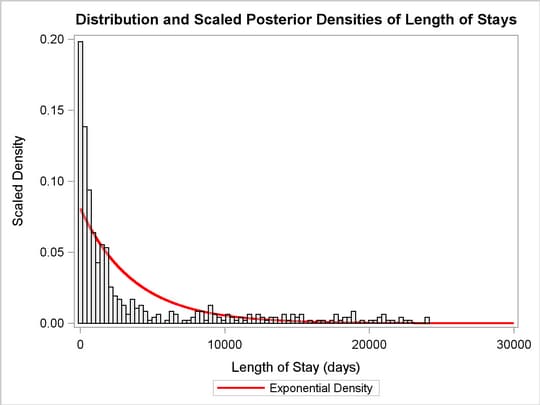
Figure 2 displays a plot that illustrates the skewness of the data. The histogram of the data is overlaid with a scaled exponential density, and you can see that a single exponential density does not fit the lower values of LOS well.

Figure 2 Length of Stay, Exponential Density

Bayesian Mixture of Exponential Model

Mixture models arise naturally when one mechanism generates data according to one model and another mechanism generates data according to a different model. In this data set, the variable that indicates which mechanism generated an observation is not recorded, and only the response variable is available. A mixture model is useful for analyzing this data set because it unveils the latent heterogeneity that arises from a latent categorical variable (Fruhwirth-Schnatter; 2006 ) .

Mixture models can be expressed as a weighted average of $\text{[math]}$ component densities. More formally, $\text{[math]}$ is said to arise from a finite mixture model with probability density function $\text{[math]}$ where

$\text{[math]}$

For all $\text{[math]}$ , $\text{[math]}$ is the component probability density function, and $\text{[math]}$ are the weights defined by the following constraints: $\text{[math]}$ and $\text{[math]}$ .

Congdon ( 2003 ) states that exponential mixture models with relatively small number of components are effective in modeling skewed LOS data. You can write a two-component exponential mixture model for LOS data with density as follows:

$\text{[math]}$

for patients $\text{[math]}$ .

There are three parameters in the density: $\text{[math]}$ , and $\text{[math]}$ . Researchers Harrison and Millard ( 1991 ) suggest the mean parameters, $\text{[math]}$ and $\text{[math]}$ , as the average LOS for the standard- and long-stay groups, respectively. In addition, $\text{[math]}$ represents an unknown fraction of patients in the standard-stay group with $\text{[math]}$ .

Suppose the following prior distributions are placed on the three parameters:

	$\text{[math]}$	$\text{[math]}$	$\text{[math]}$
	$\text{[math]}$	$\text{[math]}$	$\text{[math]}$

where $\text{[math]}$ indicates a prior distribution and $\text{[math]}$ is the density function for the inverse-gamma distribution. Priors of this type are often called diffuse priors . The $\text{[math]}$ prior expresses your lack of knowledge about the mixture proportion.

Label-switching is a common problem that arises in mixture models. It was described by as a result of the invariance of the mixture likelihood function under the relabeling of the mixture components. In an effort to remove label-switching, Harrison and Millard ( 1991 ) place an identifiability constraint that the average LOS of the standard-stay group is less than that of the long-stay group; that is, $\text{[math]}$ .

Using Bayes’ theorem, the likelihood function and prior distributions determine the posterior distribution of $\text{[math]}$ , and $\text{[math]}$ as follows:

$\text{[math]}$

PROC MCMC obtains samples from the desired posterior distribution, which is determined by the prior and likelihood specified. It does not require the form of the posterior distribution.

The following SAS statements use the prior distributions to fit the Bayesian exponential mixture model. The PROC MCMC statement invokes the procedure and specifies the input data set. The NMC= option specifies the number of posterior simulation iterations. The THIN=5 option specifies that one of every five samples is kept. The PROPCOV=QUANEW option uses the estimated inverse Hessian matrix as the initial proposal covariance matrix.

   ods graphics on;
   proc mcmc data=inputdata seed=1010 nmc=50000 thin=5 
      propcov=quanew statistics=summary;
      ods output PostSummaries = post_summ;
      parms B 100 D 6000 pi 0.5;
      prior B D ~ igamma(3/10, scale = 10/3);
      prior pi ~ uniform(0,1);
      if (B < D) then
         llike = log(pi*pdf("expo", los, B) + (1-pi)*pdf("expo", los, D));
      else
         llike = .;
      model general(llike);
   run;    
   ods graphics off;

The ODS OUTPUT statement creates an output data set post_summ used later for a graphical analysis of the fit in Figure 8 . The PARMS statement puts all three parameters $\text{[math]}$ , $\text{[math]}$ , and $\text{[math]}$ in a single block and assigns initial values to each of them. The PRIOR statements specify priors for all the parameters. Note that $\text{[math]}$ and $\text{[math]}$ can be specified with one PRIOR statement because they have the same prior distribution.

The IF-ELSE statements enable different values of LOS to have different log-likelihood functions, depending on whether the order constraint placed on the mean parameters is satisfied. The MODEL statement specifies that llike is the log likelihood for each observation in the model and is simply a missing value when the order constraint is not met.

By turning ODS Graphics on, PROC MCMC produces graphs at the end of the procedure which enable you to visually examine the convergence of the chain. See Figure 3 . Inferences should not be made if the Markov chain has not converged.

Figure 3 LOS Diagnostic Plots for $\text{[math]}$ , $\text{[math]}$ , and $\text{[math]}$

LOS Diagnostic Plots for B,D, and , continued

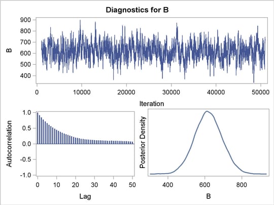
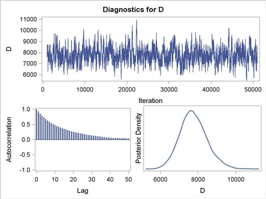
Figure 3 displays convergence diagnostic graphs for parameters $\text{[math]}$ , $\text{[math]}$ , and $\text{[math]}$ . The trace plots indicate that the chains appear to have reached stationary distributions. The chain also has good mixing and is dense.

The autocorrelation plots indicate low autocorrelation and efficient sampling. Finally, the kernel density plots show the smooth, unimodal shape of posterior marginal distributions for each parameter. If label-switching had occured, you would see jumps in the trace plots or multimodal density plots.

Figure 4 contains the "Parameters" table which lists the names of the parameters, the blocking information, the sampling method used, the starting values, and the prior distributions.

Figure 4 LOS Parameter Information

Parameters
Parameter	Sampling Method	Initial Value	Prior Distribution
B	N-Metropolis	100.0	igamma(3/10, scale = 10/3)
D	N-Metropolis	6000.0	igamma(3/10, scale = 10/3)
pi	N-Metropolis	0.5000	uniform(0,1)

The "Tuning History" table, shown in Figure 5 , displays how the tuning stage progresses for the multivariate random walk Metropolis algorithm used by PROC MCMC to generate samples from the posterior distribution. An important aspect of the algorithm is the calibration of the proposal distribution. The tuning of the Markov chain is broken into a number of phases. In each phase, PROC MCMC generates trial samples and automatically modifies the proposal distribution as a result of the acceptance rate.

The "Burn-In History" and the "Sampling History" tables show the burn-in and main phase sampling, respectively.

Figure 5 LOS Burn-In and Sampling History

Tuning History
Phase	Block	Scale	Acceptance Rate
1	1	2.3800	0.0280
2	1	1.0123	0.0700
3	1	0.5221	0.3420

Burn-In History
Block	Scale	Acceptance Rate
1	0.5221	0.3980

Sampling History
Block	Scale	Acceptance Rate
1	0.5221	0.3811

Figure 6 displays summary and interval statistics for each posterior distribution.

Figure 6 LOS MCMC Summary and Interval Statistics

The MCMC Procedure

Posterior Summaries
Parameter	N	Mean	Standard Deviation	Percentiles
Parameter	N	Mean	Standard Deviation	25%	50%	75%
B	10000	619.1	74.2261	568.9	618.3	668.3
D	10000	7752.6	721.2	7267.1	7710.4	8202.1
pi	10000	0.5638	0.0403	0.5370	0.5655	0.5916

Posterior Intervals
Parameter	Alpha	Equal-Tail Interval		HPD Interval
B	0.050	473.6	767.0	472.0	763.7
D	0.050	6418.1	9288.4	6339.5	9195.0
pi	0.050	0.4826	0.6389	0.4825	0.6387

Figure 7 reports a number of convergence diagnostics to assist in determining convergence. These are the Monte Carlo standard errors, the autocorrelations at selected lags, the Geweke diagnostics, and the effective sample sizes.

Figure 7 LOS MCMC Convergence Diagnostics

The MCMC Procedure

Monte Carlo Standard Errors
Parameter	MCSE	Standard Deviation	MCSE/SD
B	3.9598	74.2261	0.0533
D	38.2006	721.2	0.0530
pi	0.00164	0.0403	0.0408

Posterior Autocorrelations
Parameter	Lag 1	Lag 5	Lag 10	Lag 50
B	0.9150	0.6588	0.4459	0.0689
D	0.9220	0.6766	0.4760	0.0354
pi	0.5086	0.3438	0.2564	0.0267

Geweke Diagnostics
Parameter	z	Pr > \|z\|
B	0.1718	0.8636
D	-0.2669	0.7895
pi	-0.3073	0.7586

Effective Sample Sizes
Parameter	ESS	Correlation Time	Efficiency
B	351.4	28.4595	0.0351
D	356.4	28.0580	0.0356
pi	601.9	16.6129	0.0602

Figure 6 displays the marginal posterior summaries. The larger group of standard-stay patients has an average LOS of $\text{[math]}$ days relative to the smaller group of long-stay patients whose stay averages $\text{[math]}$ days. The posterior average mixture proportions are $\text{[math]}$ and $\text{[math]}$ for the standard-stay and long-stay group, respectively.

Figure 8 illustrates the scaled mixture of exponential density and the gain in model fit from the two-component exponential mixture model.

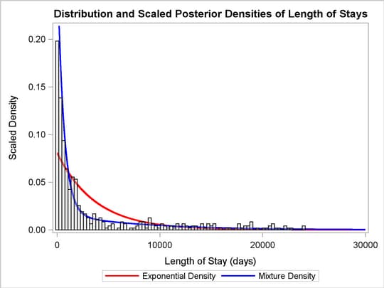
Figure 8 Length of Stay, Exponential and Mixture Density

The single-component exponential model had an average LOS of 3712 days. The mean parameters found when fitting an exponential mixture model to the standard-stay group and the long-stay group are 619 and 7752 days, respectively. The mixture distribution fits the data better than the exponential distribution, especially at the low values of LOS. Additional components could be fit and evaluated in similar methods or with information criteria.

References

Congdon, P. (2003), Applied Bayesian Modeling , John Wiley & Sons.

Fruhwirth-Schnatter, S. (2006), Finite Mixture and Markov Switching Models , Springer.

Harrison, G. and Millard, P. (1991), “Balancing Acute and Long-Term Care: The Mathematics of Throughput in Departments of Geriatric Medicine,” Meth. Infor. Medicine , 30, 221–228.

McClean, S. and Millard, P. (1993), “Patterns of Length of Stay after Admission in Geriatric Medicine: An Event History Approach,” The Statistician , 42(3), 263–274.

These sample files and code examples are provided by SAS Institute Inc. "as is" without warranty of any kind, either express or implied, including but not limited to the implied warranties of merchantability and fitness for a particular purpose. Recipients acknowledge and agree that SAS Institute shall not be liable for any damages whatsoever arising out of their use of this material. In addition, SAS Institute will provide no support for the materials contained herein.



data inputdata;
   input los @@;
   datalines;                                                                         
1671 1300   722   586   552   525  364                                                
 359  321   302   272   248   226  216
 208  182   141   141   132   120  117
 115  114   113   104   103   101   99                                          
  96   94    93    92    88    84   83
  81   79    74    70    63    62   62
  61   56    55    53    53    51   51
  50   49    36    33    33    33   29
  28   26    24    19    16    16   15
    14 9 9 5 5 3 3
     2 2 1 24028 23871 22852 22464
22317 21525 21264 21131 21077 20944 20608
20133 19583 19038 18821 18761 18742 18479
18449 18241 18128 17830 17800 17746 17285
16763 16444 15922 15226 15224 15178 14885
14744 14715 14601 14482 14174 14149 13295
13274 12850 12661 12660 12405 12300 12248
11821 11769 11577 11159 10680 10414 10393
10253 10095 9926 9722 9670 9426 9389
 9109 9004 9003 8959 8927 8583 8465
 8464 8317 8176 8156 8114 8096 7884
 7639 6552 6387 6283 6243 6155 5917
 5397 5370 5165 5007 4899 4408 4395
 4290 4282 4208 4182 4153 3855 3810
 3735 3719 3676 3467 3225 3149 3115
 2989 2933 2927 2918 2802 2746 2701
 2542 2430 2421 2380 2340 2331 2318
 2235 2209 2053 1997 1978 1923 1856
 1812 1804 1792 1757 1717 1670 1666
 1661 1615 1610 1609 1525 1481 1424
 1388 1376 1349 1302 1159 1134 1057
 1006 937 756 733 723 588 533
  522 348 212 439 188 181 141
  131 116 96 83 56 40 40
   37 36 26 23 19 14 8
20809 20319 18918 15058 13540 13446 10161
 9163 6474 5420 4584 4341 3805 3640
 3640 3578 3453 3375 3186 2756 2724
 2658 2599 2583 2416 2261 2232 2127
 2126 2035 2015 1986 1903 1897 1874
 1780 1776 1759 1752 1749 1730 1624
 1580 1552 1549 1546 1493 1472 1469
 1456 1441 1433 1428 1399 1391 1378
 1363 1359 1317 1295 1279 1262 1247
 1201 1199 1195 1182 1175 1141 1135
 1106 1049 1037 1031 1027 1006 994
  972 952 944 938 938 936 933
  897 887 880 880 863 842 806
  792 791 789 764 762 726 712
  707 706 703 697 691 687 677
   649 635 613 607 602 602 601
   594 590 576 569 552 544 544
   539 532 530 525 511 509 502
   497 477 462 453 446 443 434
   426 414 411 407 399 397 391
   375 374 370 366 365 359 357
   351 350 348 345 343 341 337
   336 336 333 330 330 310 306
   300 289 285 273 260 252 238
   231 223 219 215 197 197 197
   187 187 161 126 125 123 107
   100 93 83 58 48 37 37
  35   28    20    19     9     5    2
   2    2 22317 14006 11549 11006 8981
8402 7947  7266  6693  4408  4010 4003
1970 1857  1849  1833  1770  1769 1514
1217  956   924   611   386   280   93
;


/*-----------------------------------------------------------------
  Example: Fitting a Mixture of Exponential Distributions for
           Patients Length of Stay 
  Requires: SAS/STAT
  Version: 9.2                                                                       
  ------------------------------------------------------------------*/

** Calculates the Average number of days in hospital stays **;
proc means data = inputdata;
   ods output Summary=summ;
run;

** Creates a macro variable for the mean LOS **;
data _null_;
   set summ;
   call symputx("los_Mean",los_Mean);
run;

** Calculates the Scaled density of Exponential **;
data a;
   do x = 10 to 30000 by 1; 
      ex1 = 300*pdf("expo", x, &los_Mean); 
      output;
   end;
run;

** Merges inputdata and scaled density data set **;
data a_inputdata;
   set a inputdata;
run; 

** Template for displaying Histogram, and both scaled density plots **;
proc template;
   define statgraph sasuser.hist;
      begingraph;
      entrytitle "Distribution and Scaled Posterior Densities of Length of Stays"; 
         layout overlay / border=FALSE 
            xaxisopts=(label="Length of Stay (days)")
            yaxisopts=(label="Scaled Density");   
            seriesplot x = x y = ex1 / primary = true 
               lineattrs=(thickness = 2 color=red) 
               name = '1' legendlabel = "Exponential Density";  
            histogram los / binwidth=300 scale=proportion 
               fillattrs=(color=lightgray transparency = .6); 
            discretelegend '1'/across=2 autoalign=(center)
               location=outside;
         endlayout;
      endgraph;
   end;
run;
   
ods graphics on;   
** Create graph **;
proc sgrender data=a_inputdata template=sasuser.hist;
run;     
ods graphics off;                                             

ods graphics on;
proc mcmc data=inputdata seed=1010 nmc=50000 thin=5 
   propcov=quanew;
   ods output PostSummaries = post_summ;
   parms B 100 D 6000 pi 0.5;
   prior B D ~ igamma(3/10, scale = 10/3);
   prior pi ~ uniform(0,1);
   if (B < D) then
      llike = log(pi*pdf("expo", los, B) + (1-pi)*pdf("expo", los, D));
   else
      llike = .;
   model general(llike);
run;    
ods graphics off;  

** Creates several macro variables for calculating posterior density **;
data _null_;
   set post_summ;
   if(Parameter = "B") then do;
      b_temp = Mean;
      call symputx("Bmean",b_temp);
      end;   
   if(Parameter = "D") then do;
      d_temp = Mean;
      call symputx("Dmean",d_temp);
      end;
   if(Parameter = "pi") then do;
      pi_temp = Mean;
      call symputx("pimean",pi_temp);
      end;
run;

** Creates ex2 variable, scaled density values of mixture **;
data b;
   do x2 = 200 to 30000 by 1; 
      ex2 = 300*(&pimean*pdf("expo", x2, &Bmean) + 
              (1- &pimean)*pdf("expo", x2, &Dmean));  
      output;
   end;
run;

** Creates combined output data sets **;
data b_inputdata;
   set a b inputdata;
run;

** Template for displaying Histogram, and scaled density plots **;
proc template;                                           
   define statgraph sasuser.hist2;
      begingraph;
      entrytitle "Distribution and Scaled Posterior Densities of Length of Stays"; 
         layout overlay / border=FALSE 
            xaxisopts=(label="Length of Stay (days)")
            yaxisopts=(label="Scaled Density");   
         seriesplot x = x y = ex1 /primary = true 
            lineattrs=(thickness = 2 color=red) 
            name = '1' legendlabel = "Exponential Density";  
         seriesplot x = x2 y = ex2 /primary = true 
            lineattrs=(thickness = 2 color=blue)
            name = '2' legendlabel = "Mixture Density";
         histogram los/binwidth=300 scale=proportion 
            fillattrs=(color=lightgray transparency = .6); 
         discretelegend '1' '2'/across=2 autoalign=(center) 
            location=outside;
         endlayout;
      endgraph;
   end;
run;

ods graphics on;   
** Create graph **;
proc sgrender data=b_inputdata template=sasuser.hist2;                        
run;     
ods graphics off;

These sample files and code examples are provided by SAS Institute Inc. "as is" without warranty of any kind, either express or implied, including but not limited to the implied warranties of merchantability and fitness for a particular purpose. Recipients acknowledge and agree that SAS Institute shall not be liable for any damages whatsoever arising out of their use of this material. In addition, SAS Institute will provide no support for the materials contained herein.

Type:	Sample
Topic:	Analytics ==> Bayesian Analysis SAS Reference ==> Procedures ==> MCMC

Date Modified:	2018-05-31 10:19:33
Date Created:	2012-02-02 15:32:25

Product Family	Product	Host	Product Release		SAS Release
Product Family	Product	Host	Starting	Ending	Starting	Ending
SAS System	SAS/STAT	z/OS	9.3
		Microsoft® Windows® for x64	9.3
		Microsoft Windows 95/98	9.3
		Microsoft Windows 2000 Advanced Server	9.3
		Microsoft Windows 2000 Datacenter Server	9.3
		Microsoft Windows 2000 Server	9.3
		Microsoft Windows 2000 Professional	9.3
		Microsoft Windows NT Workstation	9.3
		Microsoft Windows Server 2003 Datacenter Edition	9.3
		Microsoft Windows Server 2003 Enterprise Edition	9.3
		Microsoft Windows Server 2003 Standard Edition	9.3
		Microsoft Windows Server 2003 for x64	9.3
		Microsoft Windows Server 2008	9.3
		Microsoft Windows Server 2008 for x64	9.3
		Microsoft Windows XP Professional	9.3
		Windows 7 Enterprise 32 bit	9.3
		Windows 7 Enterprise x64	9.3
		Windows 7 Home Premium 32 bit	9.3
		Windows 7 Home Premium x64	9.3
		Windows 7 Professional 32 bit	9.3
		Windows 7 Professional x64	9.3
		Windows 7 Ultimate 32 bit	9.3
		Windows 7 Ultimate x64	9.3
		Windows Millennium Edition (Me)	9.3
		Windows Vista	9.3
		Windows Vista for x64	9.3
		64-bit Enabled AIX	9.3
		64-bit Enabled HP-UX	9.3
		64-bit Enabled Solaris	9.3
		HP-UX IPF	9.3
		Linux	9.3
		Linux for x64	9.3
		Solaris for x64	9.3

Support

Sample 45566: Bayesian Exponential Mixture Model

Analysis

Bayesian Mixture of Exponential Model

References

Operating System and Release Information