PDF of Example | SAS/STAT Focus Area Examples

---

Analysis

Count data frequently display overdispersion and excess zeros, which motivates zero-inflated count models (Lambert; 1992 ; Greene; 1994 ) . Zero-inflated count models offer a way of modeling the excess zeros in addition to allowing for overdispersion in a standard parametric model. Zero inflation arises when one mechanism generates only zeros and the other process generates both zero and nonzero counts.

Zero-inflated models can be expressed as a two-component mixture model where one component has a degenerate distribution at zero and the other is a count model. More formally, a zero-inflated model can be written as

where

( 1 )

and where is a standard count model with mean , support , and is a mixture proportion with .

The following hypothetical data represents the number of fish caught by visitors at a state park. Variables are created for the visitor’s age and gender. Two dummy variables, FEMALE and MALE, are created to indicate the gender.

   data catch;
      input gender $ age count @@;   
      if gender = 'F' then do;
         female = 1; male = 0;
         end;
      else do;
         female = 0; male = 1;
         end;
      obs = _N_;
   datalines;
      F 54 18 M 37 0 F 48 12 M 27 0
      M 55 0 M 32 0 F 49 12 F 45 11
      M 39 0 F 34 1 F 50 0 M 52 4
      M 33 0 M 32 0 F 23 1 F 17 0
      F 44 5 M 44 0 F 26 0 F 30 0
      F 38 0 F 38 0 F 52 18 M 23 1
      F 23 0 M 32 0 F 33 3 M 26 0
      F 46 8 M 45 5 M 51 10 F 48 5
      F 31 2 F 25 1 M 22 0 M 41 0
      M 19 0 M 23 0 M 31 1 M 17 0
      F 21 0 F 44 7 M 28 0 M 47 3
      M 23 0 F 29 3 F 24 0 M 34 1
      F 19 0 F 35 2 M 39 0 M 43 6
   ;
         

Although these data appear to be a likely candidate for a ZIP model, you typically begin with a standard analysis and evaluate the evidence for overdispersion.

Bayesian Poisson Regression Model

Suppose you want to fit a Bayesian Poisson regression model for the number of fish caught with density as follows:

					( 2 )

for the surveyed park visitors.

The likelihood function for each of the counts and corresponding covariates is

( 3 )

where denotes a conditional probability density. The Poisson density is evaluated at the specified value of and corresponding mean parameter . The three parameters in the likelihood are , and , which correspond to an intercept, slope for age for females, and slope for age for males, respectively.

Suppose the following prior distributions are placed on the three parameters:

( 4 )

where indicates a prior distribution. The diffuse prior expresses your lack of knowledge about the regression parameters.

Using Bayes’ theorem, the likelihood function and prior distributions determine the posterior distribution of , and as follows:

PROC MCMC obtains samples from the desired posterior distribution, which is determined by the prior and likelihood specified. It does not require the form of the posterior distribution.

The goodness-of-fit Pearson chi-square statistic as given in McCullagh and Nelder ( 1989 ) , is calculated to assess model fit:

( 5 )

for a Poisson likelihood where with as defined in Equation 2 , is the expectation, and is the variance. If there is no overdispersion, the Pearson statistic would roughly equal the number of observations in the data set minus the number of parameters in the model.

The following SAS statements use the diffuse prior distributions to fit the Bayesian Poisson regression model and calculate the fit statistic.

   ods graphics on;
   proc mcmc data=catch seed=1181 nmc=100000 thin=10
      propcov=quanew monitor =(_parms_ Pearson);
      ods select Parameters PostSummaries PostIntervals tadpanel;
      parms beta0 0 beta1 0 beta2 0;
      prior beta: ~ normal(0,var=1000);
      mu = exp(beta0 + beta1*female*age + beta2*male*age);
      model count ~ poisson(mu);
      if obs = 1 then Pearson = 0;
      Pearson =  Pearson + ((count - mu)**2/mu);
   run;     
   ods graphics off;
          

The PROC MCMC statement invokes the procedure and specifies the input data set. The SEED= option specifies a seed for the random number generator, which guarantees the reproducibility of the random stream. The NMC= option specifies the number of posterior simulation iterations. The THIN=10 option controls the thinning of the Markov chain and specifies that one of every 10 samples is kept. The PROPCOV=QUANEW option initializes the Markov chain at the posterior mode and uses the estimated inverse Hessian matrix as the initial proposal covariance matrix in the random walk Metropolis algorithm. The MONITOR= option specifies a list of symbols (which can be either parameters or functions of the parameters in the model) for which inference is to be done. The symbol _parms_ is a shorthand for all model parameters—in this case, , , and . The symbol Pearson refers to the Pearson chi-square statistic, which is a function of the data and parameters.

The PARMS statement puts all three parameters , , and in a single block and assigns initial values to each of them. The PRIOR statement specifies priors for all the parameters. The notation beta: in the PRIOR statement is a shorthand for all variables that start with ' beta '. In this example, it includes beta0 , beta1 , and beta2 . The shorthand notation is not necessary, but it keeps your code succinct. The assignment statement for mu calculates in the Poisson model, as given in Equation 2 . The MODEL statement specifies the likelihood function for COUNT, as given in Equation 3 .

The next two lines of statements use the posterior samples of mu and the data set variable count to calculate the Pearson chi-square statistic. The IF statement resets the value of Pearson to be zero at the top of the data set (that is, when the data set variable obs is 1). As PROC MCMC cycles through the data set at each iteration, the procedure cumulatively adds the Pearson chi-square statistic over each value of count . By the end of the data set, you obtain the Pearson chi-square statistic, as defined in Equation 5 .

It is essential to examine the convergence of the Markov chains before you proceed with posterior inference in Bayesian analysis. With ODS Graphics turned on, PROC MCMC produces graphs at the end of the procedure output which allow you to visually examine the convergence of the chain. See Figure 1 . Inferences should not be made if the Markov chain has not converged.

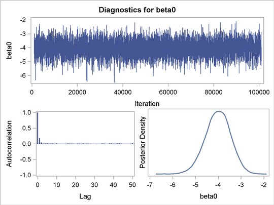
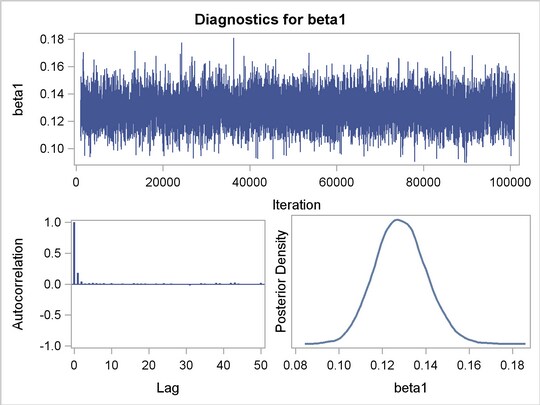
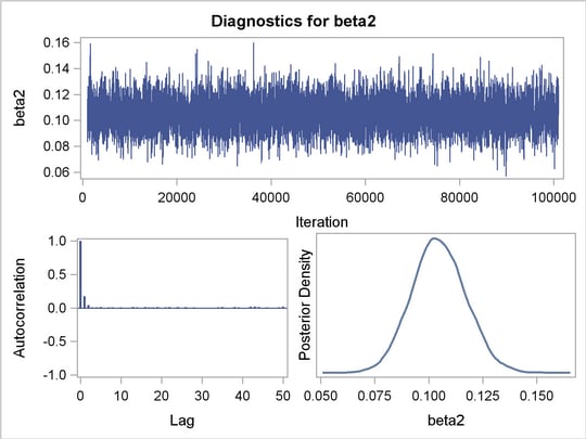
Figure 1 displays convergence diagnostic plots for , , and . The trace plots show that the mean of the Markov chain is constant over the graph and is stabilized. The chain was able to traverse the support of the target distribution, and the mixing is good. The trace plots show that the Markov chain appears to have reached stationary distributions.

The autocorrelation plots indicate low autocorrelation and efficient sampling. The kernel density plots show smooth, unimodal posterior marginal distributions for each parameter.

PROC MCMC produces formal diagnostic tests by default, but they are omitted here because an informal check on the chains, autocorrelation, and posterior density plots show desired stabilization and convergence.

The "Parameters" tables, shown in Figure 2 , lists the names of the parameters, the sampling method used, the starting values, and the prior distributions.

The MCMC Procedure

Parameters
Parameter	Sampling Method	Initial Value	Prior Distribution
beta0	N-Metropolis	0	normal(0,var=1000)
beta1	N-Metropolis	0	normal(0,var=1000)
beta2	N-Metropolis	0	normal(0,var=1000)

Figure 3 displays summary and interval statistics for each parameter’s posterior distribution. PROC MCMC also calculates the sampled value of the Pearson chi-square at each iteration and produces posterior summary statistics for it.

The MCMC Procedure

Posterior Summaries
Parameter	N	Mean	Standard Deviation	Percentiles
				25%	50%	75%
beta0	10000	-4.0186	0.5551	-4.3787	-4.0024	-3.6411
beta1	10000	0.1284	0.0117	0.1204	0.1281	0.1361
beta2	10000	0.1047	0.0125	0.0963	0.1043	0.1129
Pearson	10000	92.2674	12.2613	83.3871	90.0545	98.8112

Posterior Intervals
Parameter	Alpha	Equal-Tail Interval		HPD Interval
beta0	0.050	-5.1475	-2.9799	-5.0903	-2.9400
beta1	0.050	0.1064	0.1518	0.1065	0.1518
beta2	0.050	0.0808	0.1295	0.0799	0.1283
Pearson	0.050	74.8858	121.7	72.8727	116.1

With and three model parameters, the sampled value 92.2674 of the Pearson chi-square statistic is much greater than , providing evidence of overdispersion.

Zero inflation is a likely cause of this overdispersion. A Bayesian ZIP model accounts for the extra zeros and potentially provides a better fit to the data.

Bayesian ZIP Regression Model

You can write a Bayesian ZIP regression model for the number of fish caught as follows:

where is defined in Equation 1 , is defined in Equation 2 , and for the surveyed visitors. The model is a weighted average of the degenerate function (which places all mass at zero) and the Poisson regression.

The likelihood function for each of the counts and corresponding covariates is

( 6 )

where denotes a conditional probability density and the Poisson density is evaluated at the specified value of and corresponding mean parameter . The degenerate distribution is one when COUNT equals zero and remains zero for a COUNT value greater than zero. The four parameters in the likelihood are , , and , which correspond to an intercept, slope for age for females, slope for age for males, and the mixture proportion, respectively.

Suppose again that the three regression parameters have the same diffuse, normal priors as in Equation 4 . The mixture proportion has a uniform(0,1) prior distribution.

The Pearson chi-square statistic for the ZIP model is calculated as in Equation 5 , but now the mean and the variance respectively are

The following SAS statements use the prior distributions to fit the Bayesian ZIP regression model and calculate the Pearson chi-square statistic.

   ods graphics on;
   proc mcmc data=catch seed =1181 nmc=100000 thin=10 
      propcov=quanew monitor =(_parms_ Pearson);
      ods select Parameters PostSummaries PostIntervals tadpanel;
      parms beta0 0 beta1 0 beta2 0 eta .3;
      prior beta: ~ normal(0,var=1000);
      prior eta ~ uniform(0,1);
      mu=exp(beta0 + beta1*female*age + beta2*male*age);           
      llike=log(eta*(count eq 0) + (1-eta)*pdf("poisson",count,mu));
      model general(llike);
      if obs = 1 then Pearson = 0;
      mean = (1 - eta)*mu;
      sigma2 = (1 - eta)*mu*(1 + eta*mu);   
      Pearson =  Pearson + ((count - mean)**2/sigma2);
   run;
   ods graphics off;
          

The parameter and its starting value are added to the PARMS statement with the regression parameters and their starting values. The PRIOR statement remains the same for the regression parameters, but an additional PRIOR statement is needed for the mixture proportion.

The assignment statement for mu calculates the expected value of COUNT in the Poisson model, as given in Equation 2 . The assignment statement for llike evaluates the log density of Equation 6 . The expression (count eq 0) in llike acts as an indicator variable for the degenerate distribution ; it is one when COUNT equals zero and zero for values of COUNT greater than zero. The MODEL statement specifies that llike is the log likelihood for each observation in the model.

The Pearson chi-square statistic is calculated according to Equation 5 ; the moments are evaluated in the mean and sigma2 assignment variables.

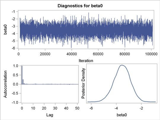
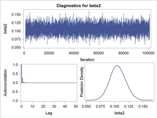
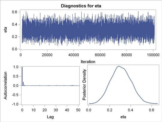
The diagnostic plots for the regression parameters and mixture proportion are illustrated in Figure 4 . They show the desired convergence, low autocorrelation, and smooth unimodal marginal posterior densities for the parameters.

Figure 5 displays the "Parameters" table for the ZIP regression model. The "Parameters" table now includes information about the mixture proportion parameter.

The MCMC Procedure

Parameters
Parameter	Sampling Method	Initial Value	Prior Distribution
beta0	N-Metropolis	0	normal(0,var=1000)
beta1	N-Metropolis	0	normal(0,var=1000)
beta2	N-Metropolis	0	normal(0,var=1000)
eta	N-Metropolis	0.3000	uniform(0,1)

Figure 6 displays summary and interval statistics for each parameter’s posterior distribution. PROC MCMC also calculates the sampled value of the Pearson chi-square at each iteration. This statistic in the Bayesian ZIP model is greatly reduced with a value of 48.8650, which suggest a much better fit compared to its value of 92.2674 in the Poisson model.

The MCMC Procedure

Posterior Summaries
Parameter	N	Mean	Standard Deviation	Percentiles
				25%	50%	75%
beta0	10000	-3.5345	0.6349	-3.9516	-3.5278	-3.0980
beta1	10000	0.1217	0.0132	0.1127	0.1214	0.1304
beta2	10000	0.1054	0.0138	0.0961	0.1051	0.1146
eta	10000	0.3074	0.0936	0.2420	0.3050	0.3719
Pearson	10000	48.8650	10.2696	41.4549	47.2985	54.4092

Posterior Intervals
Parameter	Alpha	Equal-Tail Interval		HPD Interval
beta0	0.050	-4.8193	-2.3170	-4.7908	-2.2925
beta1	0.050	0.0963	0.1485	0.0955	0.1476
beta2	0.050	0.0786	0.1331	0.0785	0.1328
eta	0.050	0.1296	0.4926	0.1290	0.4915
Pearson	0.050	33.7757	73.5911	31.6653	68.8728

Modeling the catch data set with a Bayesian ZIP regression model accounts for the zero inflation and removes the overdispersion in the Poisson regression model. Figure 6 shows the posterior parameter summaries in addition to the lowered Pearson chi-square statistic. The posterior mean of the mixture probability is for the zero-inflated component and for the Poisson regression component. The posterior parameter means of and are and , respectively. That is, an increase in one year of age is estimated to be associated with a change in the mean number of fish caught by females and males by a factor of and , respectively. For this model, choice of priors, and data set, females catch more fish with age than males.

References

Greene, W. H. (1994), Accounting for Excess Zeros and Sample Selection in Poisson and Negative Binomial Regression Models , working paper 94-10, New York University, Leonard N. Stern School of Business, Department of Economics, available at http://ideas.repec.org/p/ste/nystbu/94-10.html .

Lambert, D. (1992), “Zero-Inflated Poisson Regression Models with an Application to Defects in Manufacturing,” Technometrics , 34, 1–14.

McCullagh, P. and Nelder, J. A. (1989), Generalized Linear Models , Second Edition, London: Chapman & Hall.

---

These sample files and code examples are provided by SAS Institute Inc. "as is" without warranty of any kind, either express or implied, including but not limited to the implied warranties of merchantability and fitness for a particular purpose. Recipients acknowledge and agree that SAS Institute shall not be liable for any damages whatsoever arising out of their use of this material. In addition, SAS Institute will provide no support for the materials contained herein.

---

  
data catch;
   input gender $ age count @@;   
   if gender = 'F' then do;
      female = 1; male = 0;
      end;
   else do;
      female = 0; male = 1;
      end;
   obs = _N_;
datalines;
   F 54 18 M 37 0 F 48 12 M 27 0
   M 55 0 M 32 0 F 49 12 F 45 11
   M 39 0 F 34 1 F 50 0 M 52 4
   M 33 0 M 32 0 F 23 1 F 17 0
   F 44 5 M 44 0 F 26 0 F 30 0
   F 38 0 F 38 0 F 52 18 M 23 1
   F 23 0 M 32 0 F 33 3 M 26 0
   F 46 8 M 45 5 M 51 10 F 48 5
   F 31 2 F 25 1 M 22 0 M 41 0
   M 19 0 M 23 0 M 31 1 M 17 0
   F 21 0 F 44 7 M 28 0 M 47 3
   M 23 0 F 29 3 F 24 0 M 34 1
   F 19 0 F 35 2 M 39 0 M 43 6
;


ods graphics on;
proc mcmc data=catch seed=1181 nmc=100000 thin=10
   propcov=quanew monitor =(_parms_ Pearson);
   ods select Parameters PostSummaries PostIntervals tadpanel;
   parms beta0 0 beta1 0 beta2 0;
   prior beta: ~ normal(0,var=1000);
   mu = exp(beta0 + beta1*female*age + beta2*male*age);
   model count ~ poisson(mu);
   if obs = 1 then Pearson = 0;
   Pearson =  Pearson + ((count - mu)**2/mu);
run;     
ods graphics off;  

ods graphics on;
proc mcmc data=catch seed =1181 nmc=100000 thin=10 
   propcov=quanew monitor =(_parms_ Pearson);
   ods select Parameters PostSummaries PostIntervals tadpanel;
   parms beta0 0 beta1 0 beta2 0 eta .3;
   prior beta: ~ normal(0,var=1000);
   prior eta ~ uniform(0,1);
   mu=exp(beta0 + beta1*female*age + beta2*male*age);           
   llike=log(eta*(count eq 0) + (1-eta)*pdf("poisson",count,mu));
   model general(llike);
   if obs = 1 then Pearson = 0;
   mean = (1 - eta)*mu;
   sigma2 = (1 - eta)*mu*(1 + eta*mu);   
   Pearson =  Pearson + ((count - mean)**2/sigma2);
run;
ods graphics off;  

---

These sample files and code examples are provided by SAS Institute Inc. "as is" without warranty of any kind, either express or implied, including but not limited to the implied warranties of merchantability and fitness for a particular purpose. Recipients acknowledge and agree that SAS Institute shall not be liable for any damages whatsoever arising out of their use of this material. In addition, SAS Institute will provide no support for the materials contained herein.

This example illustrates fitting Bayesian zero-inflated Poisson (ZIP) models to zero-inflated count data with the experimental MCMC procedure.

Type:	Sample
Topic:	Analytics ==> Bayesian Analysis SAS Reference ==> Procedures ==> MCMC

Date Modified:	2012-02-03 14:30:29
Date Created:	2012-01-31 11:44:40

Operating System and Release Information

Product Family	Product	Host	Product Release		SAS Release
			Starting	Ending	Starting	Ending
SAS System	SAS/STAT	Windows 7 Ultimate x64	9.3
		Windows 7 Ultimate 32 bit	9.3
		Windows 7 Professional x64	9.3
		Windows 7 Professional 32 bit	9.3
		Windows 7 Home Premium x64	9.3
		Windows 7 Home Premium 32 bit	9.3
		Windows 7 Enterprise x64	9.3
		Windows 7 Enterprise 32 bit	9.3
		Microsoft Windows NT Workstation	9.3
		Microsoft Windows 2000 Professional	9.3
		z/OS	9.3